Your data. Your AI.
Your future.
Own them all on the new data intelligence platform


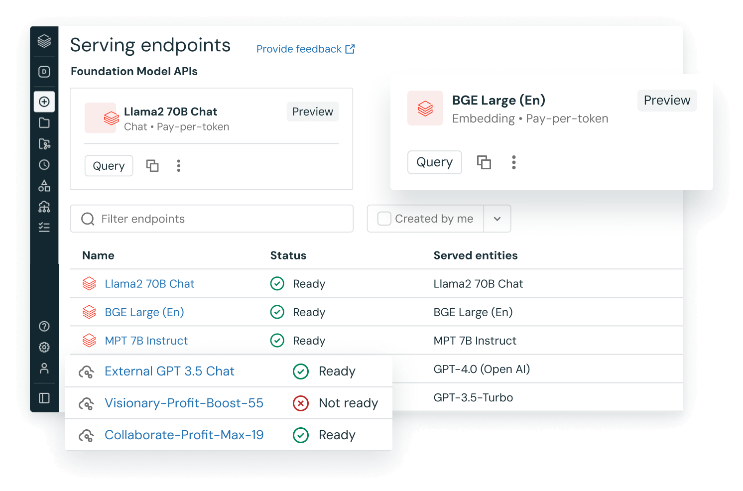
Meet DBRX, the new standard for high‑quality and efficient LLMs
DBRX, our new, open source foundation model, sets the standard for quality and efficiency. DBRX outperforms all established open models in quality benchmarks and allows you to quickly build your own custom LLM on your data.
The Databricks
Data Intelligence Platform
Databricks brings AI to your data to help you bring AI to the world.Succeed with AI
Develop generative AI applications on your data without sacrificing data privacy or control.
Democratize insights
Empower everyone in your organization to discover insights from your data using natural language.
Drive down costs
Gain efficiency and simplify complexity by unifying your approach to data, AI and governance.
Unify all your data + AI
Industry leaders are data + AI companies
Our customers achieve breakthroughs, innovate faster and drive down costs. See how you can too.


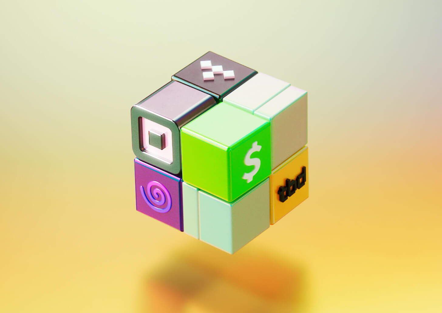
Block redefines financial services with data + AI
Plug into what you already use


Speed up success in data + AI
The Databricks Data Intelligence Platform integrates with your current tools for ETL, data ingestion, business intelligence, AI and governance. Adopt what’s next without throwing away what works.
More than meets the AI


Ready to become a data + AI company?
Take the first steps in your transformation