How Thasos Optimized and Scaled Geospatial Workloads with Mosaic on Databricks

For working with geospatial data, see this post from Databricks announcing support for Spatial SQL: Introducing Spatial SQL in Databricks: 80+ Functions for High-Performance Geospatial Analytics
Customer Insights from Geospatial Data
Thasos is an alternative data intelligence firm that transforms real-time location data from cell phones into actionable business performance insights for customers, which include institutional investors and commercial real-estate firms. Investors, for example, might want to understand metrics like aggregate foot traffic for properties owned by companies within their portfolios or to make new data-driven investment decisions. With billions of phones broadcasting their location throughout the world, Thasos gives their customers a competitive edge with powerful real-time tools for measuring and forecasting economic activity anywhere.
Challenges Scaling Geospatial Workloads
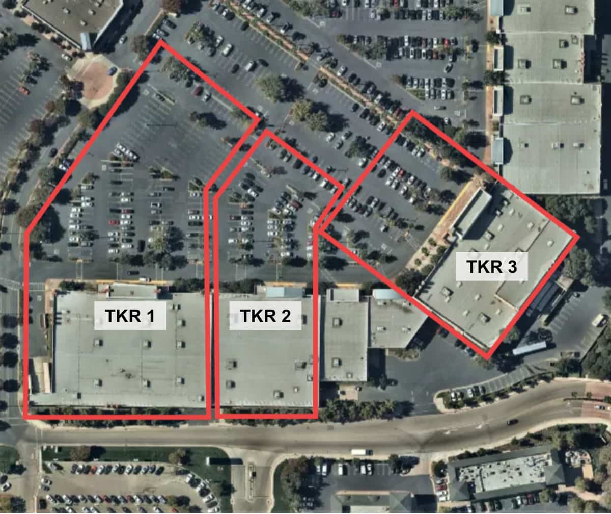
To derive actionable insights from cell phone ping data (a time series of points defined by a latitude and longitude pair), Thasos created, maintains and manages a vast collection of verified geofences – a virtual boundary or perimeter around an area of interest with metadata about each particular boundary. In geospatial terms, a simple geofence can be defined as a polygon, a sequence of latitude and longitude pairs that define the vertices of the polygon. The image below (Figure 1) is a visualization of example geofences, and the ticker symbols a piece of metadata that is critical for the intelligence products that Thasos develops.
Generating insights requires figuring out which cell phone location points fall within which geofence polygons and is called a point in polygon (PIP) join. While the challenge of scaling PIPjoins has been discussed in detail in a previous blog post, we will reiterate some key points:
- A naive approach to the PIP problem is to directly compare each of n points to m polygons (resulting in a Cartesian product).
- The individual comparisons of a point and polygon pair are a function of the complexity of the polygon; the more vertices v the polygon has, the more expensive it is to determine whether or not an arbitrary point is contained within the polygon.
- Putting these together, the complexity is O(n*m)*O(v) , which scales very poorly. What this complexity means is that the naive approach can get very expensive as the number of the points and polygons, and the complexity of polygons increases. Furthermore, there may be variance in the number of polygon vertices across rows of data (e.g., Figure 1). Consequently the O(v) multiplier across partitions of data may vary, which can cause bottlenecks in distributed processing systems.
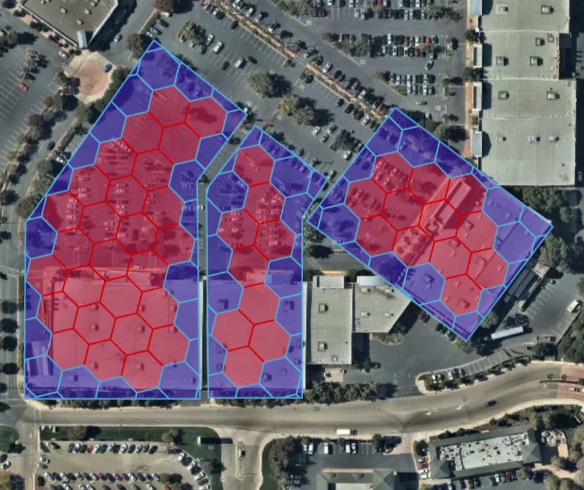
To overcome this scaling challenge, we leverage spatial index systems to reframe the PIP join as an equivalence relationship, which is computationally much less expensive than the naive approach. Geospatial index systems such as H3 and S2 create hierarchical tilings or mosaics of Earth's surface in which each tile (or cell) is assigned a unique index ID that logically groups geometries close to each other. A point is associated with a single cell (a single index ID), whereas a polygon may span over a set of cells (multiple index IDs) that are either wholly or partially contained within the polygon (Figure 2). For cells that are partially contained within a polygon, a local representation of the polygon is derived by intersecting the cell geometry with the polygon geometry yielding what is called a "chip."
When comparing the single index ID corresponding to a point, to the set of index IDs associated with the polygon there are three possible outcomes:
| Case | Conclusion |
|---|---|
| The point index ID is not contained within the set of polygon index IDs | The polygon does not contain the point |
| The point index ID is contained within the set of polygon index IDs and the cell corresponding to that index ID is completely contained within the polygon | The polygon contains the point |
| The point index ID is contained within the set of polygon index IDs and the cell corresponding to that index ID is partially contained within the polygon | We will need to compare the point with the chip (intersection of the cell geometry and the polygon) directly using contains relation - an O(v) operation |
It is important to note that the indexing of polygons is a more expensive operation than indexing point data and is a one-off cost to this approach. As geofence polygons generally do not evolve as quickly as new cell phone ping points are received, the one-time preprocessing cost is a viable compromise for avoiding expensive Cartesian products.
Scalability and Performance with Databricks and Mosaic
At Thasos, the team was working with hundreds of thousands of polygons and receiving billions of new points every day. While not all problems leveraged their full dataset, the poor scaling of the naive comparison approach was apparent with out-of-memory issues, causing failed pipelines on their warehouse. To remedy these issues, the team spatially partitioned their data, yielding stable pipelines. However, the issues of exponentially increasing processing cost and time still remained.
To address the issue of processing time, the team considered a framework that could elastically scale with their workloads, and Apache Spark was a natural choice. By leveraging more instances, the time taken to complete the pipelines could be managed. Despite the stability in time, total costs to execute the pipeline stayed relatively constant and the Thasos team was looking for a solution with better scaling, as they knew that the size and complexity of their data sources would continue to grow.
By collaborating with the Databricks team and leveraging Mosaic, the engineers at Thasos were able to reap the benefits of the optimized approach to PIP joins described in the previous section without having to implement the approach from scratch. Mosaic provided an easy to install geospatial framework with built-in functions for some of the more complicated operations (such as calculating an appropriate resolution for H3 indexing) required for the optimized PIP joins. The Thasos team identified two large pipelines appropriate for benchmarking. The first pipeline PIP joined new geofences received on a daily basis with the entire history of their cell phone ping data while the second pipeline joined newly received cell phone ping data with Census Block polygons for the purpose of data partitioning and population estimates.
| Pipeline | Spark Performance | Databricks + Mosaic Performance | Impact |
|---|---|---|---|
| #1 - Geofence PIP Pipeline | $4.33* | $1.74* | 2.5x better price/performance |
| #2 - Census Block PIP Pipeline | $130 35-40 mins | $13.08 25 mins | 10x cheaper 29-38% faster |
(*$ values are normalized)
The sizable improvements in performance provided the Thasos team confidence in the scalability of the approach and Mosaic is now an integral part of their production pipelines. Building these pipelines on the Databricks Lakehouse platform, has not only saved Thasos on cloud computing costs, but has also unlocked the opportunity to onboard data scientists on the team to develop new intelligence products and also to integrate with the broader Databricks partner ecosystem.
Getting Started
Try Mosaic on Databricks to accelerate your Geospatial Analytics on Lakehouse today and contact us to learn more about how we assist customers with similar use cases.
- Mosaic is available as a Databricks Labs repository here.
- Detailed Mosaic documentation is available here.
- You can access the latest code examples here.
Read more about our built-in functionality for H3 indexing here.
Never miss a Databricks post
What's next?

Technology
December 9, 2024/6 min read
Scale Faster with Data + AI: Insights from the Databricks Unicorns Index

News
December 11, 2024/4 min read