メインコンテンツへジャンプ
Platform blog

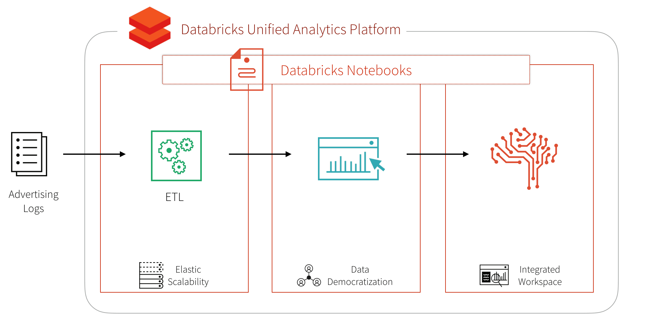
広告部門では、膨大な量の多様なマーケティングデータや Web 広告の効果を測定/分析するために、拡張性が高く柔軟なプラットフォーム・方法を必要としています。ビッグデータを活用したマーケティング効果測定(分類、クラスタリング、認識、予測、推薦などの高度な分析)によって、ビジネスの成果に結びつく、データからの深い洞察の抽出が可能となります。さまざまな種類の Web 広告の普及による多様なタイプのデータの増大に備え、Apache Sparkは、API と分散コンピューティングエンジンによってデータを容易にかつ並列に処理し、価値創出までの時間を短縮します。Databricks レイクハウスプラットフォームは、最適化されたマネージドクラウドサービスを提供し、コンピューティング資源と、共同作業のためのワークスペースのプロビジョニングを、セルフサービスで行う手段を提供します。

多くのデータサイエンティストが利用する Web サイト「Kaggle」から、広告インプレッションとクリックに関するデータ Click-Through Rate Prediction(クリック率の予測)の具体例を見ていきましょう。このワークフローの目的は、広告インプレッションの表示に対してクリックが発生するかどうかを予測する機械学習モデルを作成することです。

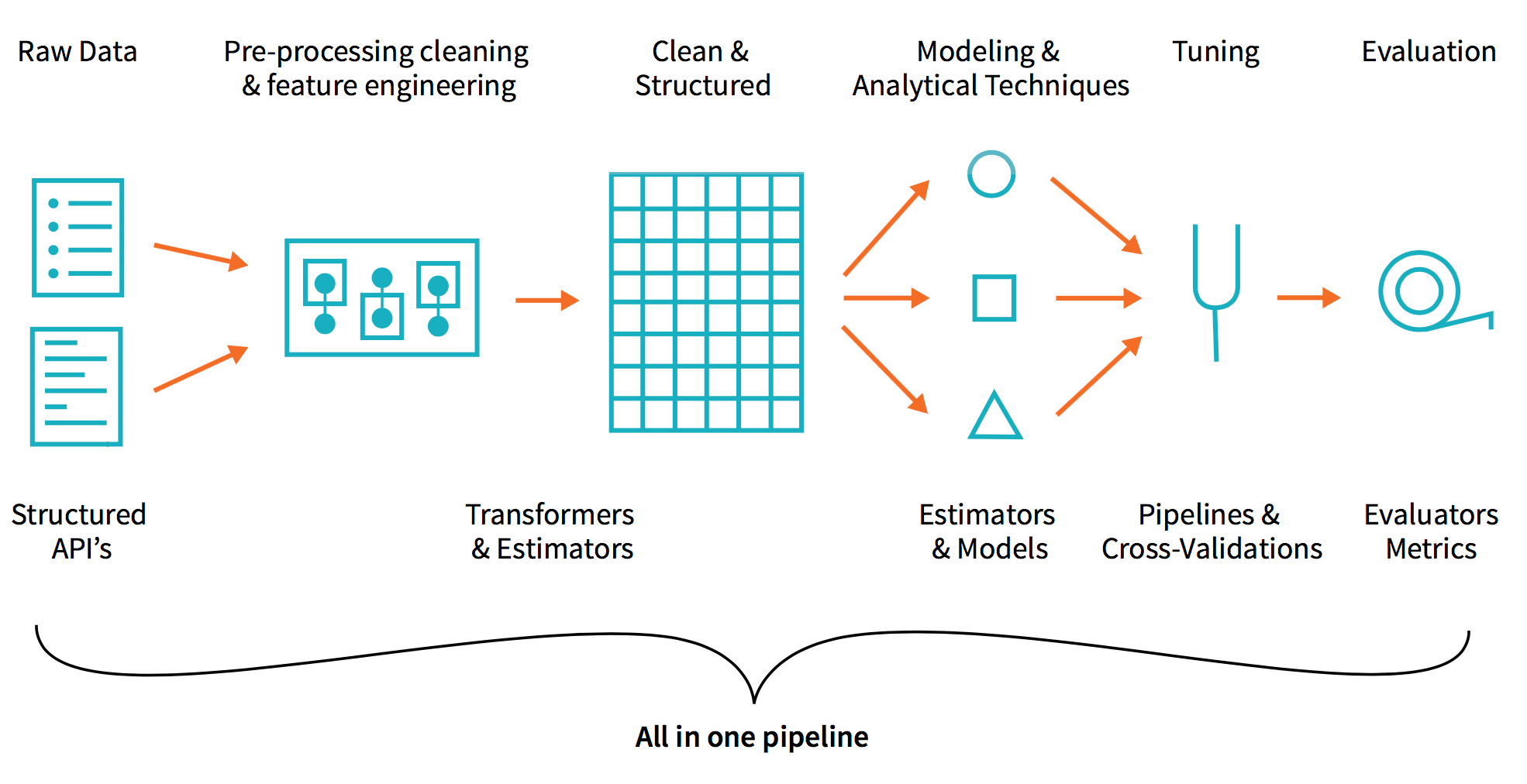
高度な広告データ分析のワークフロー構築にあたり、3 つの主要なステップを中心に解説します。

  • ETL
  • SQL などの言語を使用したマーケティングデータ探索
  • 高度な分析および機械学習

広告ログのETLプロセスを構築する

まず、データセットを AWS S3 または Microsoft Azure Blob Storage の BLOB ストレージにダウンロードします。BLOB ストレージに格納したデータは、Spark で読み込むことができます。

 
%scala // Read CSV files of our adtech dataset val df = spark.read .option("header", true) .option("inferSchema", true) .csv("/mnt/adtech/impression/csv/train.csv/") 

これで、Spark クラスタ上に、不可変なテーブル形式の分散データ構造をもつ Spark DataFrame が作成されます。推論スキーマは、.printSchema()を使用することで確認できます。

 
%scala df.printSchema() # Output id: decimal(20,0) click: integer hour: integer C1: integer banner_pos: integer site_id: string site_domain: string site_category: string app_id: string app_domain: string app_category: string device_id: string device_ip: string device_model: string device_type: integer device_conn_type: integer C14: integer C15: integer C16: integer C17: integer C18: integer C19: integer C20: integer C21: integer 

DBFS からクエリ性能を最適化するには、CSV ファイルを Parquet 形式に変換します。Parquet は、カラムナ(列指向)のファイル形式で、Spark SQL や MPP クエリエンジンを使用したビッグデータの効率的なクエリを可能にします。Parquet のための Spark の最適化について詳しくは、Github の記事 How Apache Spark performs a fast count using the Parquet metadata(Apache Spark がParquetメタデータを使用して高速カウントする方法)をご参照ください。

 
%scala // Create Parquet files from our Spark DataFrame df.coalesce(4) .write .mode("overwrite") .parquet("/mnt/adtech/impression/parquet/train.csv") 

SPARK SQL でマーケティング効果(広告ログデータなど)を探索する

Parquet ファイルに impression という名前の Spark SQL の一時ビューを作成します。Databricks ノートブックがいかに柔軟かを示すために、ノートブック内の別のセルで Python(Scalaではなく)を使用します。

 
%python # Create Spark DataFrame reading the recently created Parquet files impression = spark.read \\ .parquet("/mnt/adtech/impression/parquet/train.csv/") # Create temporary view impression.createOrReplaceTempView("impression") 

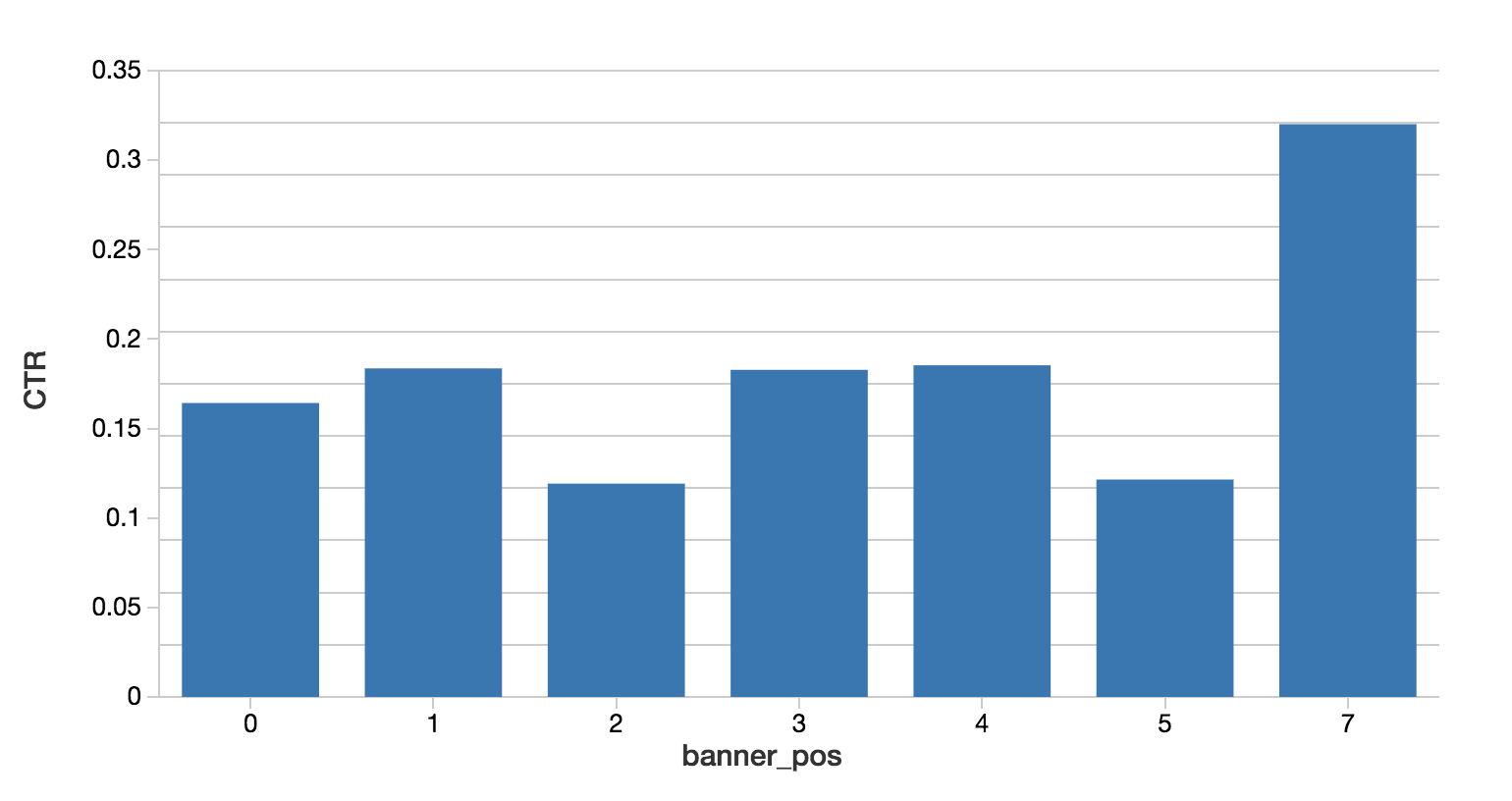
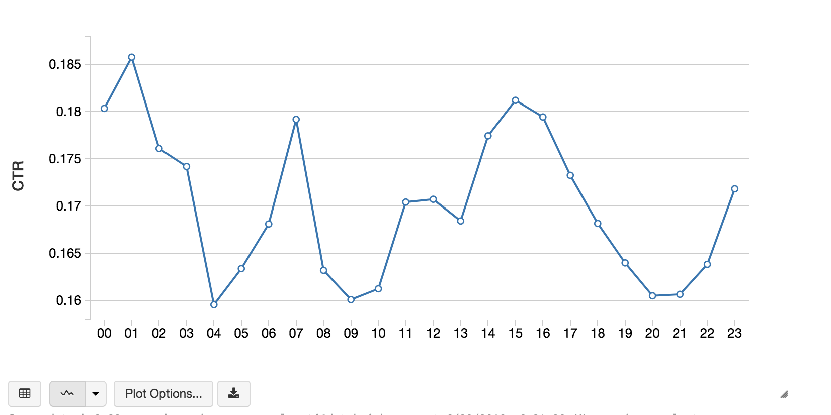
これで、使い慣れた SQL 言語を使用したデータ探索が可能になりました。Databrick sと Spark は、Scala、Python、R、SQL をサポートしています。下記のコードスニペットは、広告バナーの位置と時間帯ごとのクリック率(CTR)を計算しています。

 
%sql -- Calculate CTR by Banner Position select banner_pos, sum(case when click = 1 then 1 else 0 end) / (count(1) * 1.0) as CTR from impression group by 1 order by 1 

 
%sql -- Calculate CTR by Hour of the day select substr(hour, 7) as hour, sum(case when click = 1 then 1 else 0 end) / (count(1) * 1.0) as CTR from impression group by 1 order by 1 

クリックを予測する

データに慣れてきたら、機械学習のフェーズに進みます。このフェーズでは、データを特徴量に変換して機械学習アルゴリズムへの入力とし、予測のための学習モデルを作成します。Spark MLlib アルゴリズムは double 型の特徴ベクトルの列を入力として受け取るため、一般的に特徴量エンジニアリングのワークフローには次の事項が含まれます。

  • 数値的、カテゴリ的特徴量の特定
  • 文字列のインデックス作成
  • それらを sparse ベクトルに変換

下記のコードスニペットは、特徴量エンジニアリングのワークフローの例です。

 
# Include PySpark Feature Engineering methods from pyspark.ml.feature import StringIndexer, VectorAssembler # All of the columns (string or integer) are categorical columns maxBins = 70 categorical = map(lambda c: c[0], filter(lambda c: c[1] <= maxBins, strColsCount)) categorical += map(lambda c: c[0], filter(lambda c: c[1] <= maxBins, intColsCount)) # remove 'click' which we are trying to predict categorical.remove('click') # Apply string indexer to all of the categorical columns # And add _idx to the column name to indicate the index of the # categorical value stringIndexers = map(lambda c: StringIndexer(inputCol = c, outputCol = c + "_idx"), categorical) # Assemble the put as the input to the VectorAssembler # with the output being our features assemblerInputs = map(lambda c: c + "_idx", categorical) vectorAssembler = VectorAssembler(inputCols = assemblerInputs, outputCol = "features") # The [click] column is our label labelStringIndexer = StringIndexer(inputCol = "click", outputCol = "label") # The stages of our ML pipeline stages = stringIndexers + [vectorAssembler, labelStringIndexer] 
GBTClassiferを使用する際に、StringIndexerを使用しているにも関わらず、One Hot Encoder(OHE)を適用していないことに気づかれたかもしれません。 StringIndexer を使用している場合、カテゴリ特徴量は常に k 列のカテゴリ特徴量として保持されます。ツリーノードは、特徴量Xがカテゴリのサブセットの値を持つかどうかをテストします。StringIndexer と、OHE の両方を使用する場合は、カテゴリ特徴量は一連のバイナリ特徴量に変換されます。ツリーノードでは、特徴量 X がカテゴリ a かどうか、または、その他のカテゴリかをテストします(一対他分類)。 StringIndexer のみを使用している場合は、次の利点があります。 特徴量の選択肢が限られている。 各ノードのテストは、バイナリの 1 対他特徴量よりも表現性が高い。 OHE は表現力の低いテストであり、多くのスペースを使用するため、樹状モデルの手法には OHE を使用しないことが推奨されます。ただし、線形回帰などの非樹状モデルの手法に対しては、OHE を使用する必要があります。それ以外を使用した場合は、カテゴリに誤った順序を課することになります。 ※このセクションの内容は、Databricks のブルック・ヴェニグ(Brooke Wenig)とジョセフ・ブラッドリー(Joseph Bradley)による寄稿を元にしたものです。

ワークフローを作成したら、続いて機械学習パイプラインを作成します。

 
from pyspark.ml import Pipeline # Create our pipeline pipeline = Pipeline(stages = stages) # create transformer to add features featurizer = pipeline.fit(impression) # dataframe with feature and intermediate # transformation columns appended featurizedImpressions = featurizer.transform(impression) 

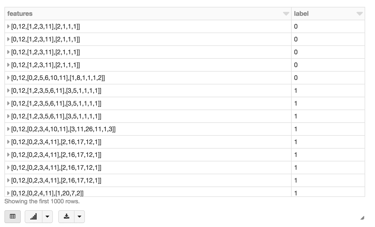
“display(featurizedImpressions.select(‘features’, ‘label’))”を使用することで、特徴量化したデータセットを視覚化できます。

次に、.randomSplit() を使用して、特徴量化したデータセットをトレーニング用とテスト用のデータセットに分割します。

 
train, test = features \ .select(["label", "features"]) \ .randomSplit([0.7, 0.3], 42) 

次に、GBTClassifier を使用して、モデルのトレーニング、予測、評価を実行します。なお、Spark MLlib でバイナリ分類問題を解決するための入門書としてスーザン・リー(Susan Li)によるMachine Learning with PySpark and MLib - Solving a Binary Classification Problemをお薦めします。

 
from pyspark.ml.classification import GBTClassifier # Train our GBTClassifier model classifier = GBTClassifier(labelCol="label", featuresCol="features", maxBins=maxBins, maxDepth=10, maxIter=10) model = classifier.fit(train) # Execute our predictions predictions = model.transform(test) # Evaluate our GBTClassifier model using # BinaryClassificationEvaluator() from pyspark.ml.evaluation import BinaryClassificationEvaluator ev = BinaryClassificationEvaluator( \\ rawPredictionCol="rawPrediction", metricName="areaUnderROC") print ev.evaluate(predictions) # Output 0.7112027059 

予測においては、ROC 曲線の AUC(下面積)のような特定の評価指標に従ってモデルを評価し、重要度別に特徴を表示することができます。このケースのAUC値は、0.7112027059でした。

まとめ

このセクションでは、Databricks の統合分析プラットフォームを使用して、クリック予測を含む広告分析をシンプルにする方法について解説しました。このプラットフォームを利用することで、クリック予測を導くための 3 つのコンポーネントである ETL、データ探索、機械学習を迅速に実行することができます。ETL、分析、機械学習パイプラインの高度な分析ワークフローを全て Databricks ノートブック内で実行することができます。

Databricks の統合分析プラットフォームを利用することで、このようなデータパイプラインに関するデータエンジニアリングの複雑さを解消し、データエンジニア、データアナリスト、データサイエンティストなど、異なるタイプのユーザーが容易に連携できるようになります。

Databricks 無料トライアル
製品一覧へ