How to Accelerate Demand Planning From 4.5 Hours to Under 1 Hour With Azure Databricks

The importance of supply chain analytics

Rapid changes in consumer purchase behavior can have a material impact on supply chain planning, inventory management, and business results. Accurate forecasts of consumer-driven demand are just the starting point for optimizing profitability and other business outcomes. Swift inventory adjustments across distribution networks are critical to ensure supply meets demand while minimizing shipping costs for consumers. In addition, consumers redeem seasonal offers, purchase add-ons and subscriptions that affect product supply and logistics planning.

Supply chain analytics at ButcherBox

ButcherBox faced extremely complex demand planning as it sought to ensure inventory with sufficient lead times, meet highly-variable customer order preferences, navigate unpredictable customer sign-ups and manage delivery logistics. It needed a predictive solution to address these challenges, adapt quickly and integrate tightly with the rest of its Azure data estate.

“Though ButcherBox was cloud-born, all our teams used spreadsheets,” said Jimmy Cooper, Head of Data, ButcherBox. “Because of this, we were working with outdated data from the moment a report was published. It’s a very different world now that we’re working with Azure Databricks.”

How ButcherBox streamlined supply chain analytics

ButcherBox uses Azure Databricks to generate its Demand Plan. When Azure Data Factory (ADF) triggers the Demand Plan run, Azure Databricks processes supply chain data from Azure Data Lake, vendor data and Hive caches. New outputs are stored in a data lake, then Azure Synapse updates Demand Plan production visualizations.

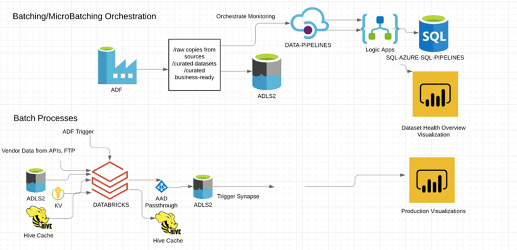
ButcherBox leverages Azure Databricks to ingest all real-time streams of raw data from vendors, internal sources and historical data. Azure Databricks reconciles this data into item, box and distribution levels for users to view demand for the upcoming year. This data is then used for retention modeling, and pushed to Azure Synapse for historical comparison.

Apache Spark SQL in Azure Databricks is designed to be compatible with Apache Hive. ButcherBox uses Hive to cache data from CSV files and then processes the cached data in Azure Databricks, enabling Demand Plan calculation times to decrease from 4.5 hours to less than one hour. This enabled an updated Demand Plan to be available for business users every morning to aid decision-making. Ingestion of these data streams also created trustworthy datasets for other processes and activities to consume. These new tools and capabilities helped ButcherBox quickly understand and adjust to changes in member behavior, especially in the midst of he COVID-19 pandemic.

Create your first demand forecast using Azure Databricks

To get started using Azure Databricks for demand forecasts, download this sample notebook and import it into your Azure Databricks workspace.

Step 1: Load Store-Item Sales Data
Our training dataset is five years of transactional data across ten different stores. We’ll define a schema, read our data into a DataFrame and then create a temporary view for subsequent querying.

Step 2: Examine data
Aggregating the data at the month level, we can observe an identifiable annual seasonality pattern, which grows over time. We can optionally restructure our query to look for other patterns such as weekly seasonality and overall sales growth.

Step 3: Assemble historical dataset
From our previous loaded data, we can build a Pandas DataFrame by querying the “train” temporary view and then remove any missing values.

Step 4: Build model

Based on exploration of the data, we will want to set model parameters in accordance with the observed growth and seasonal patterns. As such, we opted for a linear growth pattern and enabled the evaluation of weekly and yearly seasonal patterns. Once our model parameters are set, we can easily fit the model to the historical, cleansed data.

Step 5: Use a trained model to build a 90-day forecast

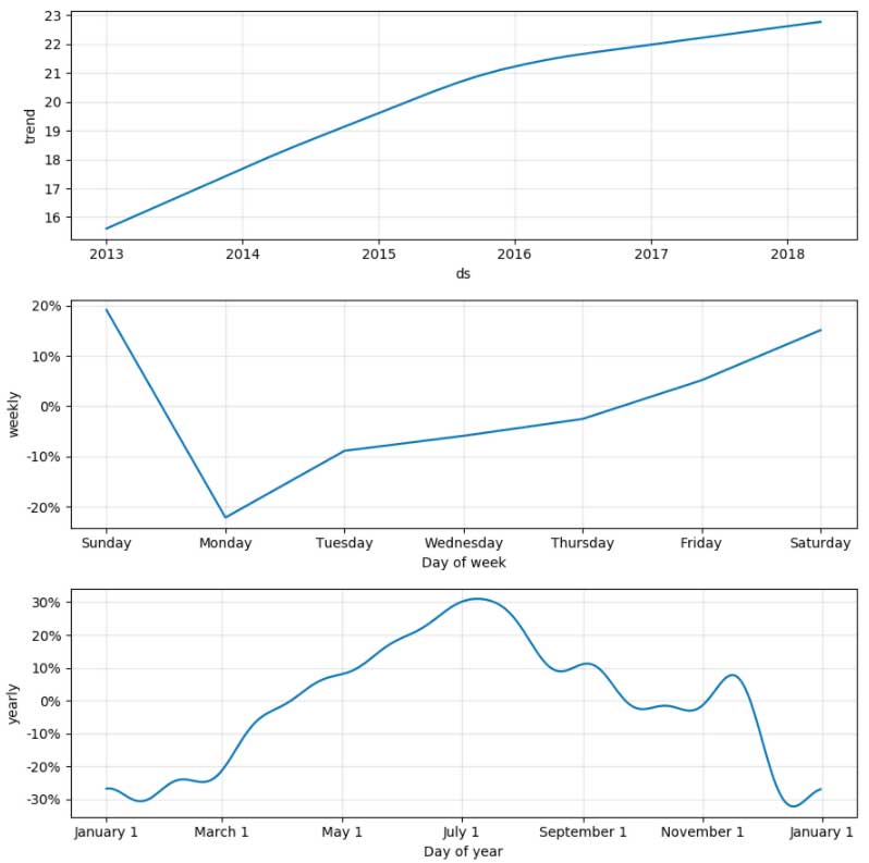
Since our model is trained, we can use it to build a forecast similar to the one ButcherBox uses in their Demand Plan. This can be done quickly using historical data as shown below.

Once we predict over the future dataset, we can produce general and seasonal trends in our model as graphs (also shown below).

Learn more by joining an Azure Databricks event and get started right away with this 3-part training series.