Efficiently Building ML Models for Predictive Maintenance in the Oil and Gas Industry With Databricks

Halliburton is an oil field services company with a 100-year-long proven track record of best-in-class oilfield offerings. With operations in over 70 countries, Halliburton provides services related to exploration, development and production of oil and natural gas. Success and increased productivity for our company and our customers is heavily dependent on the data we collect from the subsurface and during all phases of the production life cycle.

At Halliburton, petabytes of historical data about drilling and maintenance activities have been collected for decades. A huge amount of time has been spent on data collection, cleaning, transformation and feature engineering in preparation for data modelling and machine learning (ML) tasks. We use ML to automate operational processes, conduct predictive maintenance and gain insights from the data we have collected to make informed decisions.

One of our biggest data-driven use cases is for predictive maintenance, which utilizes time-series data from hundreds of sensors on equipment at each rig site, as well as maintenance records and operational information from various databases. Using Apache Spark on Azure Databricks, we can easily ingest, merge and transform terabytes of data at scale, helping us gain meaningful insights regarding possible causes of equipment failures and their relations to operational and run-time parameters.

In this blog, we discuss tools, processes and techniques that we have implemented to get more value from the extensive amounts of data using Databricks.

Analytics life cycle

Halliburton follows the basic analytics development life cycle with some variations to specific use cases. The whole process has been standardized and automated as much as possible, either through event-triggered pipeline runs or scheduled jobs. Yet, the whole workflow still provides the flexibility for some unusual scenarios.

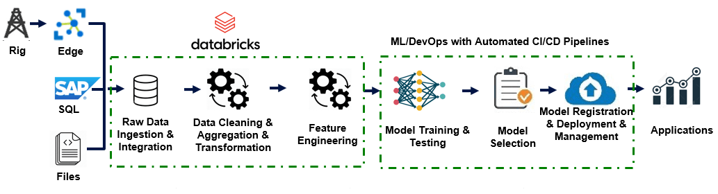
With thousands of rigs for different customers globally, each rig contains lots of tools equipped with sensors that are collecting information in real time. Large amounts of historical data collected over the past 20-30 years has been collected and stored in a variety of formats and systems, such as text files, pdf files, pictures, excel files and parquet files in SAP system, on-premise SQL databases and on network drives\local machines. For each project, data scientists, data engineers and domain experts work together to identify the different data sources, and then collect and integrate the data into the same platform.

Due to the variety of sources and varying quality of the data, data scientists spend over 80% of their time cleaning, aggregating, transforming and eventually performing feature engineering on the data. After all of this hard work, various modeling methods are explored and experimented with. The final model is selected based on a specific metric for each use case. Most of the time, the metrics chosen are directly related to the economic impact.

Once the model is selected, it can be deployed either through Azure Container Service, Azure Kubernetes Service or Azure Web App Services. After the model is deployed, it can be called and utilized in applications. However, this is not the end of the analytics life cycle. Monitoring the model performance to detect any model performance drifting over time is an essential part too. The ground truth data (after-the-fact data) flows into the system, goes through the data ingestion, data cleaning/aggregation/transformation and feature engineering. It is then stored in the system for monitoring the overall model performance or for future usage. The overall data volume is huge. However, the data for each individual equipment or well is relatively small. The data cleaning, aggregation and transformation are applied on the equipment level most of the time. Thus, if the data is partitioned by equipment number or by well, a Databricks cluster with a large number of nodes and a relatively small size for each node provides great performance boosts.

Data sources and data quality

Operational data is recorded in the field from hundreds of sensors at each rig site from the equipment belonging to different product service lines (PSLs) within Halliburton. This data is stored in a proprietary format called ADI and eventually parsed into parquet files. The amount of parquet data from one PSL could easily exceed 1.5 petabytes of historic data. With more real-time sensors and data from edge devices being recorded, this amount is expected to grow exponentially.

Configuration, maintenance and other event-related data in the field have been collected as well. These types of data are normally stored in SQL databases or entered on SAP. For example, over 5 million maintenance records have been collected in less than 2.5 years. External data has been leveraged for use when it is necessary and available, including weather related, geological and geophysical data.

Before we can analyze the vast amounts of data, it has to be merged and cleaned. At Halliburton, customized Python and PySpark libraries were developed to help us in the following ways:

• Merging un-synchronized time-series datasets acquired at different sample rates efficiently.
• Aggregating high-frequency time series data at lower frequency time intervals efficiently using user-defined aggregation functions.
• Analyzing and handling missing data (categorical or numerical) and implementing statistical techniques to fill them in.
• Efficiently detecting outliers based on thresholds, percentiles and optional deletion or replacement by statistical values

Data ingestion: Delta Lake for schema evolution, update and merge ("Upsert") capabilities

A lot of legacy data with evolving schema has been ingested into the system. The data from various sources fused and stitched together have duplicate records. For these issues, Databricks Delta Lake schema evolution and update/merge/upsert capabilities are great solutions to store such data.

The schema evolution functionality can be set with the following configuration parameter:

```python
spark.sql("set spark.databricks.delta.schema.autoMerge.enabled = true")
```

As a simple example, if incoming data is stored in the dataframe "new_data" and the Delta table archive is located in the path "delta_table_path", then the following code sample would merge the data using the keys "id", "key1" and "datetime" to check for existing records with matching keys before inserting the incoming data.

```python
from delta.tables import *
deltaTable = DeltaTable.forPath(spark, delta_table_path)

deltaTable.alias("events").merge(
    new_data.alias("updates"),
    “events.id = updates.id AND
    events.key = updates.key1 AND
    events.datetime = updates.datetime”) \
    .whenNotMatchedInsertAll()\
.execute()
```

Pandas UDF utilization

Spark performs operations row by row, which is slow for certain operations. For example, filling in the missing values for all of the sensors for each equipment, from the corresponding previous value, if it is available, or from the corresponding next available value, took hours with the Spark native window function `pyspark.sql.last('col_i', ignorenulls=[True]).over(win)` to perform the operation for one of our projects. Most of the time, it ended up with an out-of-memory error message. That was a pain point for the project. While searching online for ways to improve the operation, in one of the blogs introducing Spark windows function, someone mentioned `pandas_udf`, which turned out to be a powerful way to speed up the operation.

A Pandas user-defined function, also known as vectorized UDF, is a user-defined function that uses Apache Arrow to transfer data and utilize Pandas to work with the data. This blog is a great resource to learn more about utilizing `pandas_udf` with Apache Spark 3.0.

```python
col_list = col_sel  # a list of columns to fill in the missing values
def fill_pdf(pdf: pd.DataFrame) -> pd.DataFrame:
  for col_i in col_list:
    pdf.loc[:, col_i] = pdf[[col_i]].ffill().bfill()
  return pdf

processed_df = raw_df.groupBy('pumpID').applyInPandas(fill_pdf,schema=bldr_combined_adi_sap_fill.schema)
```

Feature engineering for large time-series datasets

Dealing with large amounts of time-series data from hundreds of sensors at each rig site can be challenging in terms of processing the data efficiently to extract features that could be useful for ML tasks.

We usually analyze time-series data acquired by sensors in fixed-length time windows during periods of activity in which we like to look at aggregated sensor amplitude information (min, max, average, etc.) and frequency domain features (peak frequency, signal-to-noise, wavelet transforms, etc.).

We make heavy use of the distributed computing features of Spark on Databricks to extract features from large time-series datasets.

As a simple example, let's consider time-series data coming from two sensor types; "sensor\*1" and "sensor\*2" are amplitudes acquired at various times ("time" column). The sensors belong to vehicle transmissions identified by "trans_id", which are powered by engines denoted by "engine_type" and drive pumps denoted by "pump_id". In this case, we already tagged the data into appropriate fixed-length time windows in a simple operation in which the window ID is in column "time_window".

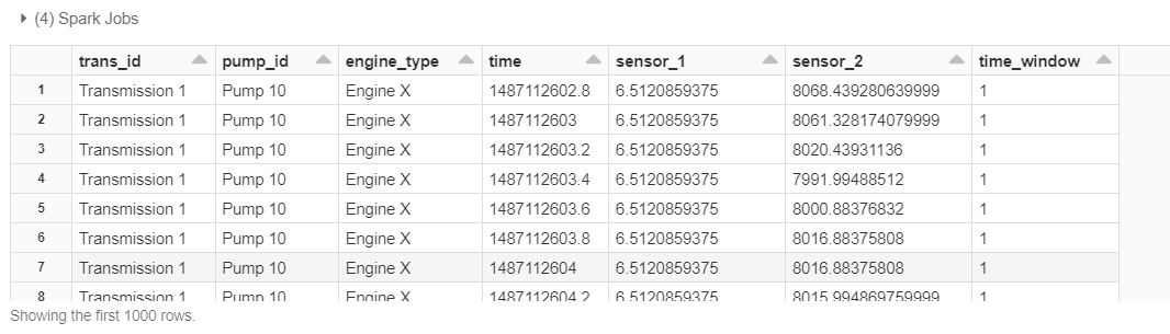
For each time window for each transmission, pump and engine grouping, we first collect the time-series data from both sensors in a tuple-like 'struct' data type:

```python
import pyspark.sql.functions as f

group_columns = ['trans_id', 'pump_id', 'engine_type', 'time_window']
process_columns = ['time', 'sensor_1', 'sensor_2']
exprs = [f.collect_list(f.struct("time", cols)).alias(cols) for cols in process_columns]
agg_df = input_df.groupBy(group_columns).agg(*exprs)
```

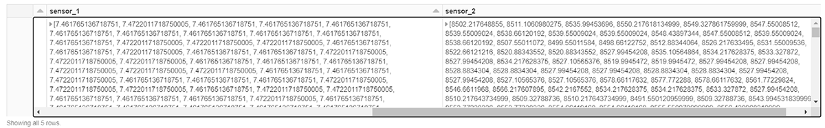
This gives us a tuple of time-amplitude pairs for each sensor in each window as shown below:

Since the ordering of the tuples is not guaranteed by the "collect_list" aggregate function due to the distributed nature of Spark, we sort these collected tuples in increasing time order using a PySpark UDF and output the sorted amplitude values:

```python
import operator

def sort_time_arrays(l):
    res = sorted(l, key=operator.itemgetter(0))
    y = [item[1] for item in res]
    return y

sort_udf = f.udf(sort_time_arrays,t.ArrayType(t.DoubleType()))

for cols in process_columns:
    agg_df = agg_df.withColumn(cols, sort_udf(cols))
```

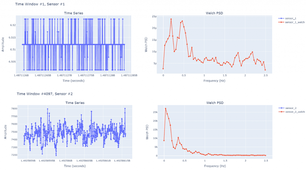
Any signal processing function can now be applied to these sensor amplitude arrays for each window efficiently using PySpark or Pandas UDFs. In this example, we extract the Welch Power Spectral Density (Welch PSD) for each time-window, and in general, this UDF can be replaced by any function:

```python
from scipy import signal

def welch(x):
    fs=1/time_interval_sel
    freq,psd=signal.welch(x,fs,nperseg=128)
    freq = freq.tolist()
    psd = psd.tolist()
    y = freq + psd
    return y

welch_udf = f.udf(welch, t.ArrayType(t.DoubleType()))
process_cols = ['sensor_1', 'sensor_2']

for col_i in process_cols:
    agg_df = agg_df.withColumn(col_i+"_freq", welch_udf(f.col(col_i)))
```

The resulting data frame contains frequency domain Welch PSD extractions for each sensor in each time window:

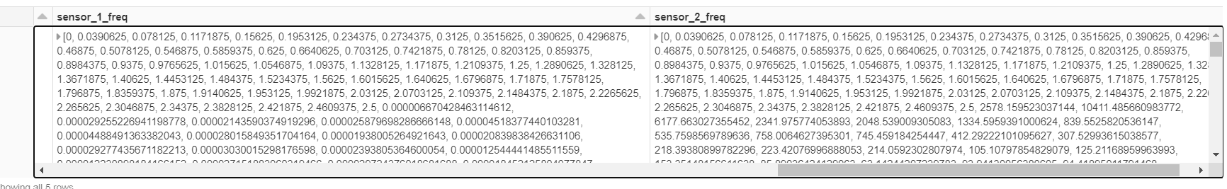
Below are some examples of the plotted time-series data and corresponding Welch PSD results for multiple windows for the two different sensors. We may choose to further extract the peak frequencies, spectral roll-off and spectral centroid from the Welch PSD results to use as features in ML tasks for predictive maintenance.

Utilizing the concepts above, we can efficiently extract features from extremely large time series datasets using Spark on Databricks.

Model Development, management and performance monitoring

Model development and model management is a big part of the analytics life cycle. At Halliburton, prior to using MLOps, the models and the corresponding environment files were stored in blob storage with certain name conventions, and a .csv file was used to track all of the model specific information. This caused a lot of confusion and errors when more and more models/experiments were tested out.

So, an MLOps application has been developed by the team to manage the whole flow in an automatic fashion. Essentially, the MLOps application links the 3 key elements: model development, model registration and model deployment, and runs them through DevOps pipelines automatically. The triggers to run the whole process are either by a code commit to a specific branch on the centralized git repo, or by updates to the dataset in the linked datastore. The whole process standardizes ML development/ deployment process, drastically reducing the ML project life cycle time with quick delivery and updates. It frees up the team to focus on differentiating value-added work, and at the same time, boosts collaboration and cooperation and provides clear project history tracking, making the analytics development across the company more sustainable.

Summary

The Databricks platform has enabled us to utilize petabytes of time series data in a manageable way. We have used Databricks to:

• Streamline the data ingestion process from various sources and efficiently store the data using Delta Lake.
• Transform and manipulate data for use in ML in an efficient and distributed manner.
• Help prepare and automate data pipelines for use in our MLOps platform.

These have helped our organization make efficient data-driven decisions that increase success and productivity for Halliburton and our customers.

Watch the Data + AI Summit Talk