High Scale Geospatial Processing With Mosaic

Breaking through the scale barrier (discussing existing challenges)

At Databricks, we are hyper-focused on supporting users along their data modernization journeys.

A growing number of our customers are reaching out to us for help to simplify and scale their geospatial analytics workloads. Some want us to lay out a fully opinionated data architecture; others have developed custom code and dependencies from which they do not want to divest. Often customers need to make the leap from single node to distributed processing to meet the challenges of scale presented by, for example, new methods of data acquisition or feeding data-hungry machine learning applications.

In cases like this, we frequently see platform users experimenting with existing open source options for processing big geospatial data. These options often have a steep learning curve which can pose challenges unless customers have already developed a familiarity with a given framework's best practices and patterns for deploying and using. Users struggle to achieve the required performance through their existing geospatial data engineering approach and many want the flexibility to work with the broad ecosystem of spatial libraries and partners.

While design decisions always come with a tradespace, we have listened to and learned from our customers while building a new geospatial library called Mosaic. The purpose of Mosaic is to reduce the friction of scaling and expanding a variety of workloads, as well as serving as a repository for best practice patterns developed during our customer engagements.

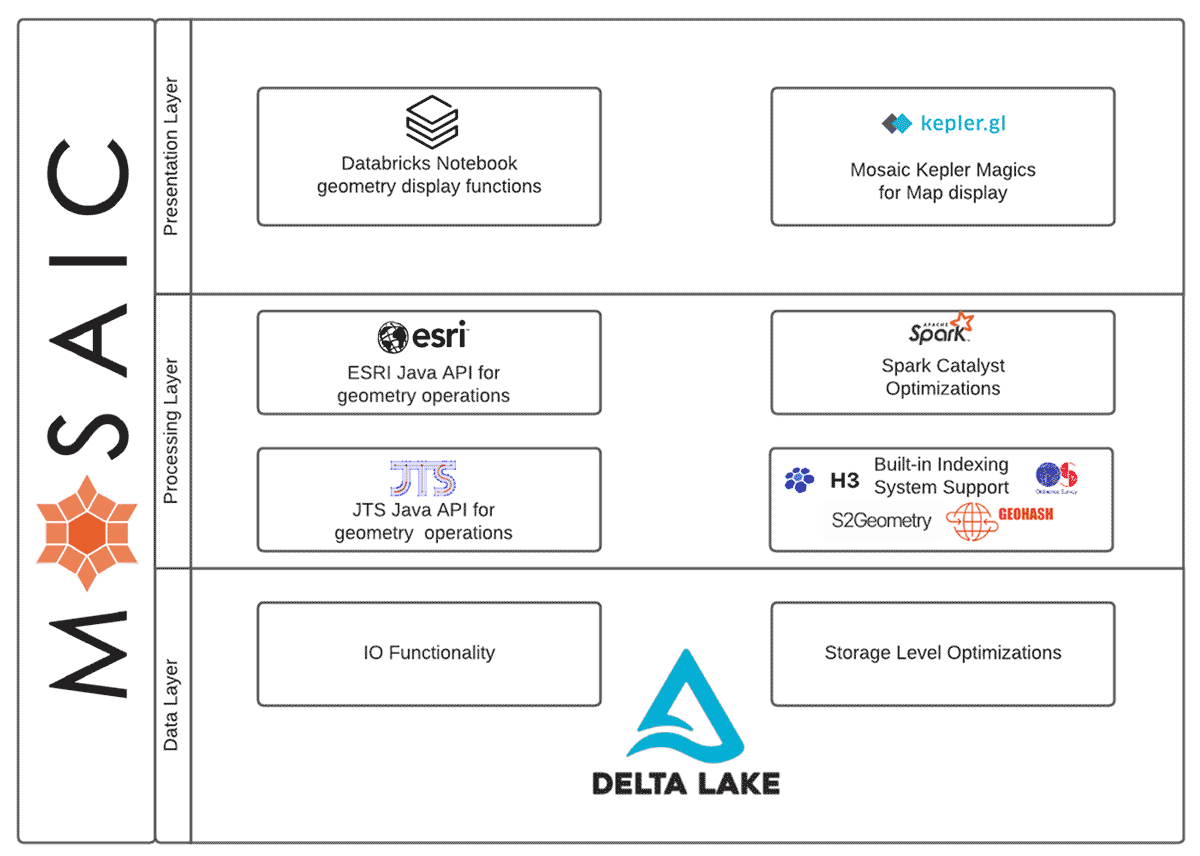
At its core, Mosaic is an extension to the Apache Spark™ framework, built for fast and easy processing of very large geospatial datasets. Mosaic provides:

• A geospatial data engineering approach that uniquely leverages the power of Delta Lake on Databricks, while remaining flexible for use with other libraries and partners
• High performance through implementation of Spark code generation within the core Mosaic functions
• Many of the OGC standard spatial SQL (ST_) functions implemented as Spark Expressions for transforming, aggregating and joining spatial datasets
• Optimizations for performing spatial joins at scale
• Easy conversion between common spatial data encodings such as WKT, WKB and GeoJSON
• Constructors to easily generate new geometries from Spark native data types and conversion to JTS Topology Suite (JTS) and Environmental Systems Research Institute (Esri) geometry types
• The choice among Scala, SQL and Python APIs

Embrace the ecosystem

Our idea for Mosaic is for it to fit between Spark and Delta on one side and the rest of the existing ecosystem on the other side. We envision Mosaic as a library that brings the know-how of integrating geospatial capabilities into systems able to benefit from a high level of parallelism. Popular frameworks such as Apache Sedona or GeoMesa can still be used alongside Mosaic, making it a flexible and powerful option even as an augmentation to existing architectures.

On the other hand, systems designed without additionally required geospatial tools can be migrated onto data architectures with Mosaic, thus leveraging high scalability and performance with minimal effort due to support of multiple languages and a unified APIs. The added value being that since Mosaic naturally sits on top of Lakehouse architecture, it can unlock AI/ML and advanced analytics capabilities of your geospatial data platform.

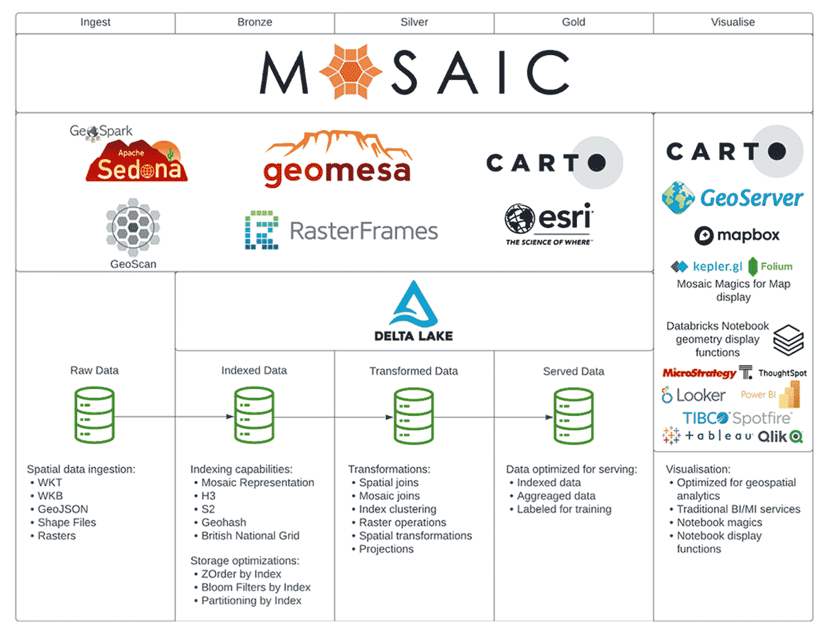
Finally, solutions like CARTO, GeoServer, MapBox, etc. can remain an integral part of your architecture. Mosaic aims to bring performance and scalability to your design and architecture. Visualization and interactive maps should be delegated to solutions better fit for handling that type of interactions. Our aim is not to reinvent the wheel but rather to address the gaps we have identified in the field and be the missing tile in the mosaic.

Using proven patterns

Mosaic has emerged from an inventory exercise that captured all of the useful field-developed geospatial patterns we have built to solve Databricks customers' problems. The outputs of this process showed there was significant value to be realized by creating a framework that packages up these patterns and allows customers to employ them directly.

You could even say Mosaic is a mosaic of best practices we have identified in the field.

We had another reason for choosing the name for our framework. The foundation of Mosaic is the technique we discussed in this blog co-written with Ordnance Survey and Microsoft where we chose to represent geometries using an underlying hierarchical spatial index system as a grid, making it feasible to represent complex polygons as both rasters and localized vector representations.

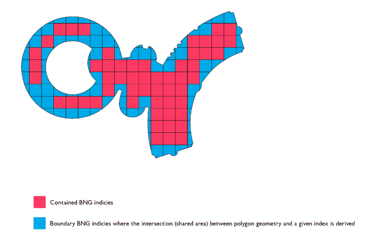
The motivating use case for this approach was initially proven by applying BNG, a grid-based spatial index system for the United Kingdom to partition geometric intersection problems (e.g. point-in-polygon joins). While our first pass of applying this technique yielded very good results and performance for its intended application, the implementation required significant adaptation in order to generalize to a wider set of problems.

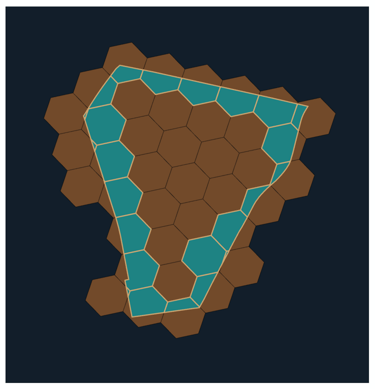
This is why in Mosaic we have opted to substitute the H3 spatial index system in place of BNG, with potential for other indexes in the future based on customer demand signals. H3 is a global hierarchical index system mapping regular hexagons to integer ids. By their nature, hexagons provide a number of advantages over other shapes, such as maintaining accuracy and allowing us to leverage the inherent index system structure to compute approximate distances. H3 comes with an API rich enough for replicating the mosaic approach and, as an extra bonus, it integrates natively with the KeplerGL library which can be a huge enabler for rendering spatial content within workflows that involve development within the Databricks notebook environment.

Mosaic has been designed to be applied to any hierarchical spatial index system that forms a perfect partitioning of the space. What we refer here to as a perfect partitioning of the space has two requirements:

1. no overlapping indices at a given resolution
2. the complete set of indices at a given resolution forms an envelope over observed space

If these two conditions are met we can compute our pseudo-rasterization approach in which, unlike traditional rasterization, the operation is reversible. Mosaic exposes an API that allows several indexing strategies:

• Index maintained next to geometry as an additional column
• Index separated within a satellite table
• Explode original table over the index through geometry chipping or mosaic-ing

Each of these approaches can provide benefits in different situations. We believe that the best tradeoff between performance and ease of use is to explode the original table. While this increases the number of rows in the table, the approach addresses the within-row skew and maximizes opportunity to utilize techniques like Z-Order and Bloom Filters. In addition, due to simpler geometries being stored in each row, all geospatial predicates will run faster because they will operate on simple local geometry representations.

The focus of this blog is on the mosaic approach to indexing strategies that take advantage of Delta Lake. Delta Lake comes with some very useful capabilities when processing big data at high volumes and it helps Spark workloads realize peak performance. Z-Ordering is a very important Delta feature for performing geospatial data engineering and building geospatial information systems. In simple terms, Z ordering organizes data on storage in a manner that maximizes the amount of data that can be skipped when serving queries.

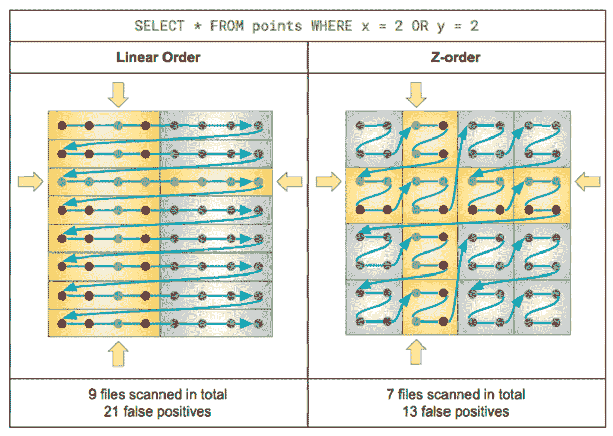
Geospatial datasets have a unifying feature: they represent concepts that are located in the physical world. By applying an appropriate Z-ordering strategy, we can ensure that data points that are physically collocated will also be collocated on storage. This is advantageous when serving queries with high locality. Many geospatial queries aim to return data relating to a limited local area or co-processing data points that are near to each other instead of the ones that are far apart.

This is where indexing systems like H3 can be very useful. H3 ids on a given resolution have index values close to each other if they are in close real-world proximity. This makes H3 ids a perfect candidate to use with Delta Lake's Z-ordering.

Making Geospatial on Databricks simple

Today, the sheer amount of data processing required to address business needs is growing exponentially. Two consequences of this are clear - 1) data does not fit into a single machine anymore and 2) organizations are implementing modern data stacks based on key cloud-enabled technologies.

The Lakehouse architecture and supporting technologies such as Spark and Delta are foundational components of the modern data stack, helping immensely in addressing these new challenges in the world of data. However, when it comes to using these tools to run large scale joins with highly complex geometries, this can still be a daunting task for many users.

Mosaic aims to bring simplicity to geospatial processing in Databricks, encompassing concepts that were traditionally supplied by multiple frameworks and were often hidden from the end users, thus generally limiting users' ability to fully control the system. The aim is to provide a modular system that can fit the changing needs of users, while applying core geospatial data engineering techniques which serve as the baseline for follow-on processing, analysis, and visualization. Mosaic supports runtime representations of geometries using either JTS or Esri types. With simplicity in mind Mosaic brings a unified abstraction for working with both geometry packages and is optimally designed for use with Dataset APIs in Spark. Unification is very important as switching between these two packages (both have their pros and cons and fit better different use cases) shouldn't be a complex task and it should not affect the way you build your queries.

%python
from mosaic import enable_mosaic
spark.conf.set(
  "spark.databricks.mosaic.geometry.api",
  "JTS"
)
enable_mosaic(spark, dbutils)

left_df.join(
  right_df,
  on=["h3_index"],
  how="inner"
).groupBy(
  key
).count()

%python
from mosaic import enable_mosaic
spark.conf.set(
  "spark.databricks.mosaic.geometry.api",
  "ESRI"
)
enable_mosaic(spark, dbutils)

left_df.join(
  right_df,
  on=["h3_index"],
  how="inner"
).groupBy(
  key
).count()

The approach above is intended to allow easy switching between JTS or Esri geometry packages for different tasks, though not to be mixed within the same notebook. We strongly recommend that you use a single Mosaic context within a single notebook and/or single step of your pipelines.

Bringing the indexing patterns together with easy-to-use APIs for geo-related queries and transformations unlocks the full potential of your large scale system by integrating with both Spark and Delta.

%python
df = df.withColumn(
  "index", mosaic_explode(col("shape"))
)
df.write.format("delta").save(location)

%sql
CREATE TABLE table_name 
  USING DELTA
  LOCATION location
 
OPTIMIZE table_name 
  ZORDER BY (index.h3)  

Diagram 8: Mosaic explode in combination with Delta Z-ordering

This pseudo-rasterization approach allows us to quickly switch between high speed joins with accuracy tolerance to high precision joins by simply introducing or excluding a WHERE clause.

%python
# rasterized query
# faster but less precise
left_df.join(
  right_df,
  on=["index.h3"],
  how="inner"
).groupBy(
  key
).count()

%python
# detailed query
# slower but more precise
left_df.join(
  right_df,
  on=["index.h3"],
  how="inner"
).where(
  col("is_core") ||
   st_contains(col("chip"), col("point"))
).groupBy(
  key
).count()

Why did we choose this approach? Simplicity has many facets and one that gets often overlooked is the explicit nature of your code. Explicit is almost always better than implicit. Having WHERE clauses determine behavior instead of using configuration values leads to more communicative code and easier interpretation of the code. Furthermore, code behavior remains consistent and reproducible when replicating your code across workspaces and even platforms.

Finally, if your existing solutions leverage H3 capabilities, and you do not wish to restructure your data, Mosaic can still provide substantial value through simplifying your geospatial pipeline. Mosaic comes with a subset of H3 functions supported natively.

%python
df.withColumn(
  "indices", polyfill(col("shape"))
)

%python
df.withColumn(
  "index", point_index_geom(col("point"))
)

Accelerating pace of innovation

Our main motivation for Mosaic is simplicity and integration within the wider ecosystem; however, that flexibility means little if we do not guarantee performance and computational power. We have evaluated Mosaic against 2 main operations: point in polygon joins and polygon intersection joins. In addition we have evaluated expected performance for the indexing stage. For both use cases we have pre-indexed and stored the data as Delta tables. We have run both operations before using ZORDER optimization and after to highlight the benefits that Delta can bring to your geospatial processing efforts.

For polygon-to-polygon joins, we have focused on a polygon-intersects-polygon relationship. This relationship returns a boolean indicator that represents the fact of two polygons intersecting or not. We have run this benchmark with H3 resolutions 7,8 and 9, and datasets ranging from 200 thousand polygons to 5 million polygons.

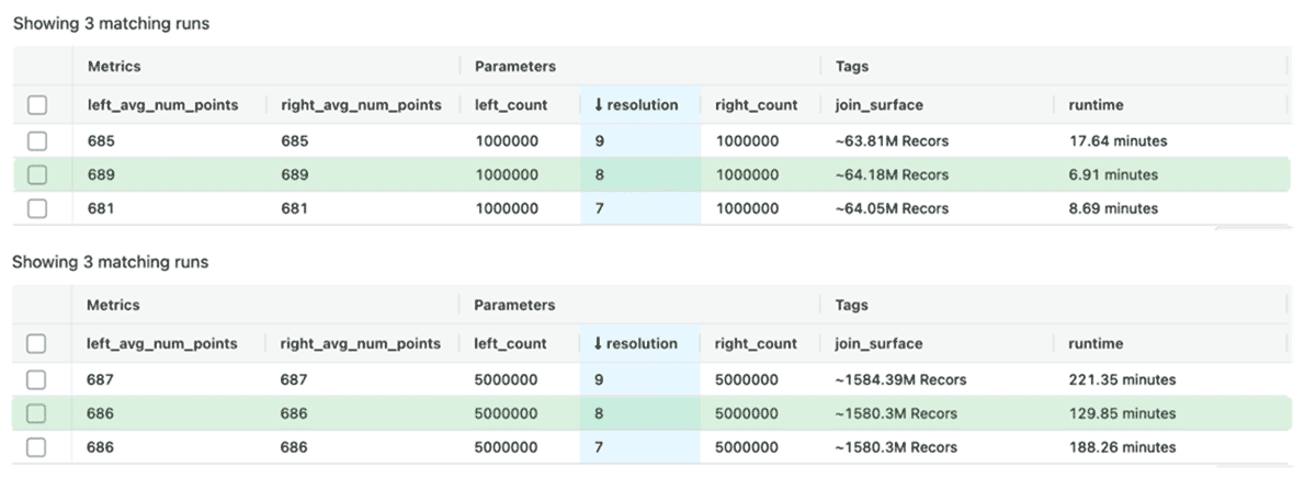
When we compared runs at resolution 7 and 8, we observed that our joins on average have a better run time with resolution 8. Most notably the largest workload of 5 million polygons joined against 5 million polygons resolution in over 1.5 billion matches ran in just over 2 hours on resolution 8 while it took about 3 hours at resolution 7. Choosing the correct resolution is an important task. If we select a resolution that is too coarse (lower resolution number) we risk of under-representing our geometries which leads to situations where geometrical data skew was not addressed and performance will degrade. If we select resolution that is too detailed (higher resolution number) we risk over-representing our geometries which leads to a high data explosion rate and performance will degrade. Striking the right balance is crucial and in our benchmarks it led to ~30% runtime optimization which highlights how important it is to have an appropriate resolution. The average number of vertices in both our datasets ranges from 680 to 690 nodes per shape - demonstrating that the Mosaic approach can handle complex shapes at high volumes.

When we increased the resolution to 9 we observed a decrease in performance - this is due to over-representation problems - using too many indices per polygon will result in too much time wasted on resolving index matches and will slow down the overall performance. This is why we have added capabilities to Mosaic that will analyze your dataset and indicate to you the distribution of the number indices needed for your polygons.

%python
from mosaic import MosaicAnalyzer

analyzer = MosaicAnalyzer()
optimal_resolution = analyzer.get_optimal_resolution(geoJsonDF, "geometry")
optimal_resolution  

Diagram 14: Determining the optimal resolution in Mosaic

For the full sets of benchmarks please refer to the Mosaic documentation page where we discuss the full range of operations we ran and provide an extensive analysis of the obtained results.

Building an atlas of use cases

With Mosaic we have achieved the balance of performance, expression power and simplicity. And with such balance we have paved the way for building end to end use cases that are modern, scalable, and ready for future Databricks product investments and partnerships across the geospatial ecosystem. We are working with customers across multiple industry verticals and we have identified many applications of Mosaic in the real world domains. Over the next months we will build solution accelerators, tutorials and examples of usage. Mosaic github repository will contain all of this content along with existing and follow-on code releases. You can easily access Mosaic notebook examples using Databricks Repos and kickstart your modern geospatial data platform - stay tuned for more content to come!

Getting started

Try Mosaic on Databricks to accelerate your Geospatial Analytics on Lakehouse today and contact us to learn more about how we assist customers with similar use cases.

• Mosaic is available as a Databricks Labs repository here.
• Detailed Mosaic documentation is available here.
• You can access the latest code examples here.
• You can access the latest artifacts and binaries following the instructions provided here.