In Part 1 of this LLM blog post series, we use the MosaicML platform to train vanilla GPT-3 models up to 1.3B params, and show how to cut training times down to hours with strong multi-node scaling. We also discover that larger models can train more efficiently than smaller models on modern hardware, and that a 10x in parameter count may only result in ~5x the training time.

Large language models (LLMs) like OpenAI’s GPT-3, Google’s PaLM, and NVIDIA’s Megatron have taken the world by storm with their impressive language understanding and generation capabilities. These results, however, hide the countless headaches and long hours faced by machine learning engineers when trying to train these models at scale. These challenges include the algorithmic aspects of training (choosing the right dataset size, model size, avoiding loss spikes, etc.), systems concerns (models and optimizers that can’t fit within memory), and the sheer logistics of coordinating large clusters of GPUs (orchestrating multi-node training, minimizing communication bottlenecks, and dealing with hardware failures).
To address these challenges, a user interested in training LLMs has to implement a wide variety of techniques—from activation checkpointing to micro-batching to gang scheduling—all of which are difficult to integrate correctly into a complex training pipeline. And even when all this is done, the final training run is expected to be slow and expensive, only within the reach of the largest and best-resourced organizations in the world. Between complexity and cost, not many people attempt to train LLMs.
At MosaicML, one of our goals is to reduce the difficulties of training these large models. As a first step towards that goal, we investigated the time and cost it would take to pretrain different members of the GPT-3 model family using the MosaicML platform. This is Part 1 in a series of blog posts that will build up towards training LLMs at the largest scales studied today, and present our recipe for a MosaicGPT model that dramatically reduces the time, cost, and complexity to train.
For Part 1, we took the commonly used HuggingFace GPT-2 model and edited the model settings to match GPT-3 configurations ranging from 125 million to 1.3 billion parameters (See Table 1). We then profiled the training speed using our Composer training library and different counts of NVIDIA A100-40GB GPUs. What we found is that even with this simple baseline, pretraining billion-parameter transformers can be done within a matter of hours and a budget of a few thousand dollars, and can be done efficiently at scale! And using MosaicML’s tools makes the process a lot easier.

Training large models with MosaicML
Training large GPT models with Composer is fast and easy, thanks to built-in features such as a HuggingFace model wrapper, efficient distributed training, and automatic gradient accumulation.
For each training run, we:
- Wrote a short YAML file specifying a HuggingFace GPT model with appropriate hyperparameters.
- Launched a run using Composer and our MosaicML training platform (coming soon!).
- Scaled up to multi-node training simply by changing the # of GPUs requested.
Throughout the process of scaling up, there was no need to worry about distributed training details, modify the global batch size, or adjust the gradient accumulation steps to fit in memory. The MosaicML platform handles all the details for us, and allows us to run the exact same training workload on any system configuration.
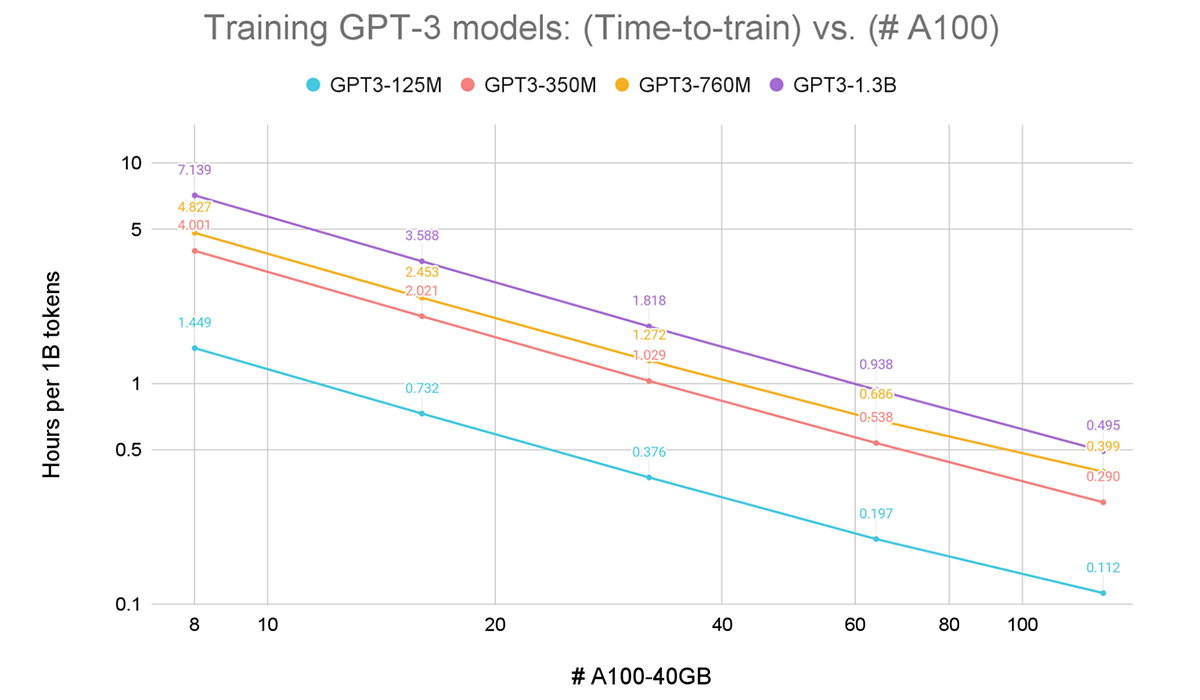
In Figure 1, we see that training these GPT models with Composer and vanilla data parallelism exhibits impressive performance. We are able to achieve near-linear strong scaling from 8x to 128x A100s. For all runs, we used a standard A100 cluster that mirrors the ones offered by major cloud providers – with NVSwitch within each node and 800Gbps RoCE interconnect across nodes.
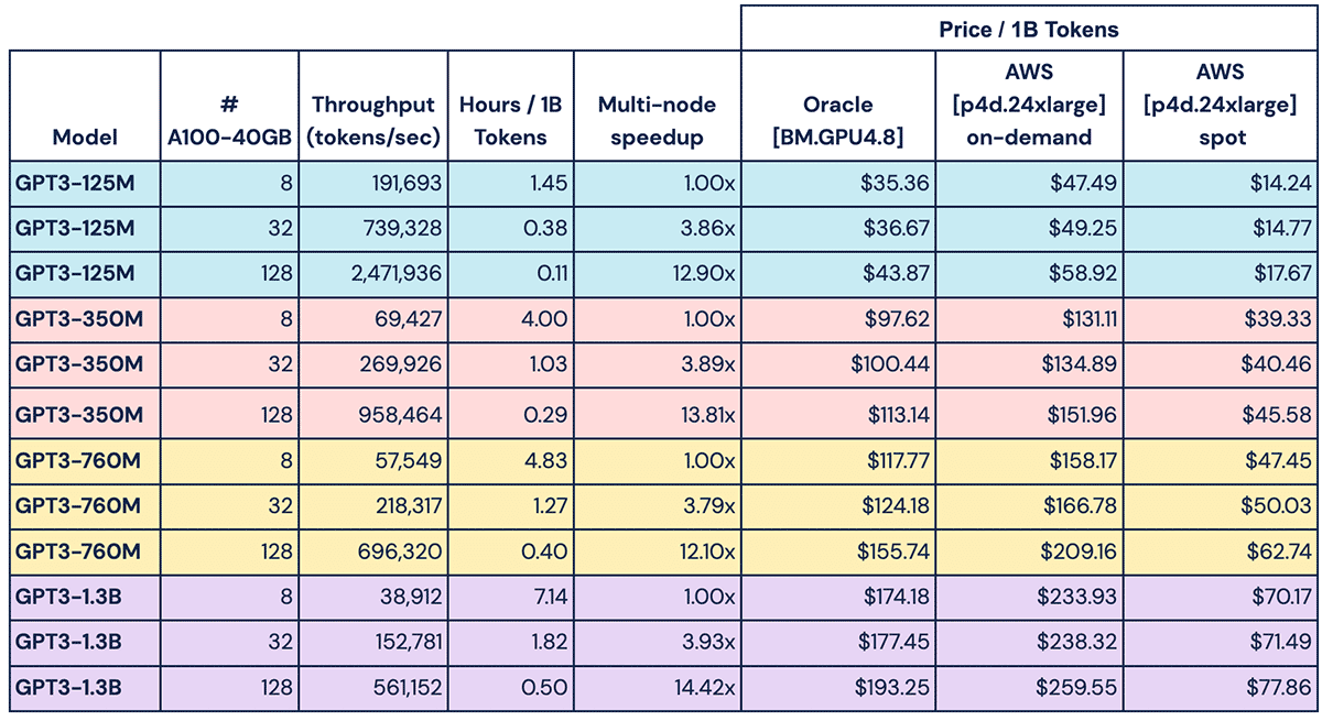
We also find that the times and costs to train these models are well within reach of both academic labs and enterprise ML engineers. For example, according to the Chinchilla paper from DeepMind, compute-optimal training of a GPT3-1.3B should use roughly 20 billion tokens. On a single node with 8xA100, we find this would take around 6 days and cost between $1400-$4600, depending on the cost of compute. In Table 2 we extrapolate some prices based on public hourly rates from Oracle and AWS.
But because we see linear scaling, we can increase our GPU count and dramatically reduce the time-to-train with only a slight increase in the total cost. For that same 1.3B model, if we train on 32xA100 we can get the job done in 1.5 days, or if using 128xA100 just 10 hours. Those are 3.9x and 14.4x speedups on 4x and 16x devices, respectively! See Table 2 for more details. The takeaway is: if your compute provider makes it possible, scaling to more nodes is worth it because you get much faster training times with minimal increase in total compute.

The Blessing of Dimensionality: It’s worth it to train at scale

Originally, we thought that scaling to larger models would mean skyrocketing compute costs, but this isn’t exactly what we found. Surprisingly, increasing the number of parameters by 10x does not necessarily mean that the model will take 10x longer to train. Comparing the runs for GPT3-125M to GPT3-1.3B, we see that training time increased by only ~5x, which means that there was a ~2x gain in training efficiency due to higher GPU utilization!
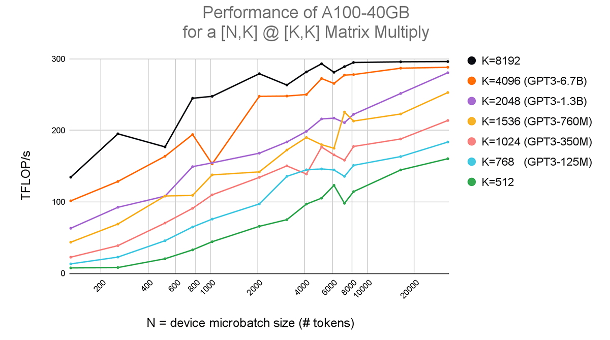
To understand why this is the case, consider the blocks of a Transformer model which contain several matrix multiplications of the form (BS, MSL, K) @ (K, K) where BS is the batch size, MSL is the max sequence length, and K is the model dimension size. This matrix multiply happens at each of the Q, K, V and output transforms, as well as twice in the feedforward layer, with some slight variations in the final dimension size but generally the same form. We profile the speed of this operation on a single A100 GPU, and for simplicity, we condense the first two dimensions BS * MSL into a single value N that can be thought of as “the number of tokens in each device’s forward pass”, or the device microbatch size.
Figure 3 shows that as we increase the model dimension K and the device microbatch size N, the throughput of the GPU in TFLOPs (trillion floating point operations per second) increases significantly, even at a fixed N. This partly explains why the GPT3-1.3B model, with a model dimension of K=2048 (purple) trains more efficiently than the GPT3-125M model with a model dimension of K=768 (blue). But what about N? In general the device microbatch size is tuned automatically by Composer and depends on the system config, but for our GPT workloads above, it was usually around N~=8192 tokens.
The takeaway here is that on modern hardware like NVIDIA A100s, it’s actually better for utilization to train models with large hidden dimensions (wider layers). This leads us to believe that scaling to the next set of models, such as GPT3-6.7B and GPT3-13B, will lead to even higher utilization. This also means that compute estimates for larger models should not be made by extrapolating on parameter count alone, as they will likely be overestimates.
The other piece of good news is that there are benefits to be reaped from extra GPU memory. When training the 1.3B param model, we had to enable activation checkpointing—where intermediate activations computed during the forward pass are not cached for the backward pass—to reduce memory usage. This comes with the overhead of having to redo the forward pass, decreasing training throughput. With higher memory-capacity devices like the A100-80GB, or sharding techniques like ZERO, we could disable activation checkpointing and gain that performance back (~1.33x).
What’s Next?
As mentioned above, these results are just Part 1 of our LLM series. In Part 2 we will demonstrate how to train larger models in the multi-billion parameter range (GPT3-2.7B, GPT3-6.7B, and beyond) using the ZERO sharding strategies, and how to enable this effortlessly with Composer. We will also explore optimizations beyond the vanilla HuggingFace GPT model, such as efficient attention kernels, and show how this can greatly reduce training time and costs. Finally, in later chapters we will apply algorithmic methods such as the ones we developed for ResNet+ImageNet, and release our MosaicGPT recipe for efficient language modeling. Stay tuned and follow us on Twitter, join our Slack community, or experiment with Composer for your training tasks!
