In our previous blog post, we showed how we used the MosaicML platform, Streaming datasets, and the Composer library to train a Stable Diffusion model from scratch for less than $50,000. Now, we do a deep dive into the technical details behind this speedup, demonstrating how we were able to replicate the Stable Diffusion 2 base model in just 6.8 days.
Try out our code here!
Many organizations require high-performing large AI models tailored to their specific use cases. However, training such models is often prohibitively time-consuming and expensive, requiring vast amounts of computation and expertise. This is where MosaicML comes in: we provide a comprehensive solution that simplifies and accelerates the process of training these models.
In our previous blog post, we announced that we have trained a diffusion model comparable to Stable Diffusion 2 from scratch for $47.7k. In this post, we dive into the technical details to highlight how we achieved an 8x speedup/cost reduction from the number reported by StabilityAI and a 3x cost reduction over our own baseline. All of our code is open source and easy to modify for custom use cases. If you're interested in learning more about our stack, please contact us for a demo.
Accelerating Training
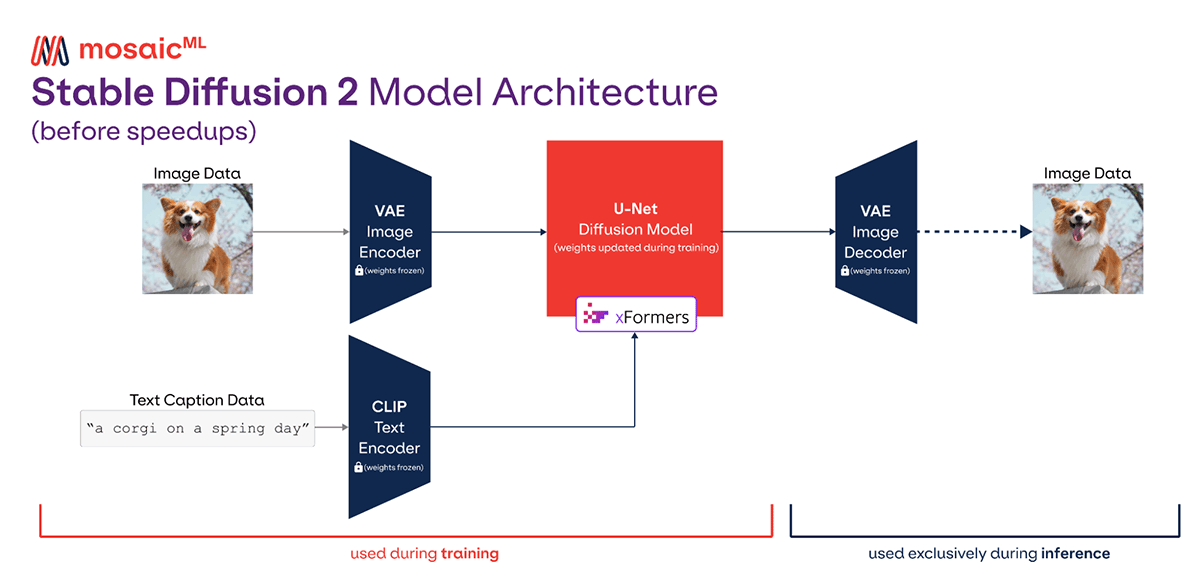
We've introduced a variety of techniques, from fusions to sharding strategies, that dramatically speed up training and lower costs by almost 3x.
xFormers FlashAttention
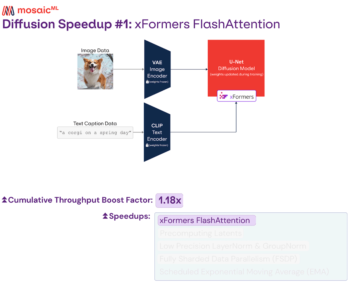
The attention layers in the Stable Diffusion architecture can be slow with a naive implementation, so most codebases use faster implementations that rely on fused kernels. In our stack, we leverage xFormers FlashAttention.
While this was enabled in our original blog post, we found an issue with the usage that resulted in extra memory being consumed on rank 0. After fixing this bug, we were able to increase our device microbatch size1 from 4 to 8. This yielded a sizable speedup, since A100s are more efficient at larger matrix sizes.
Precomputing Latents
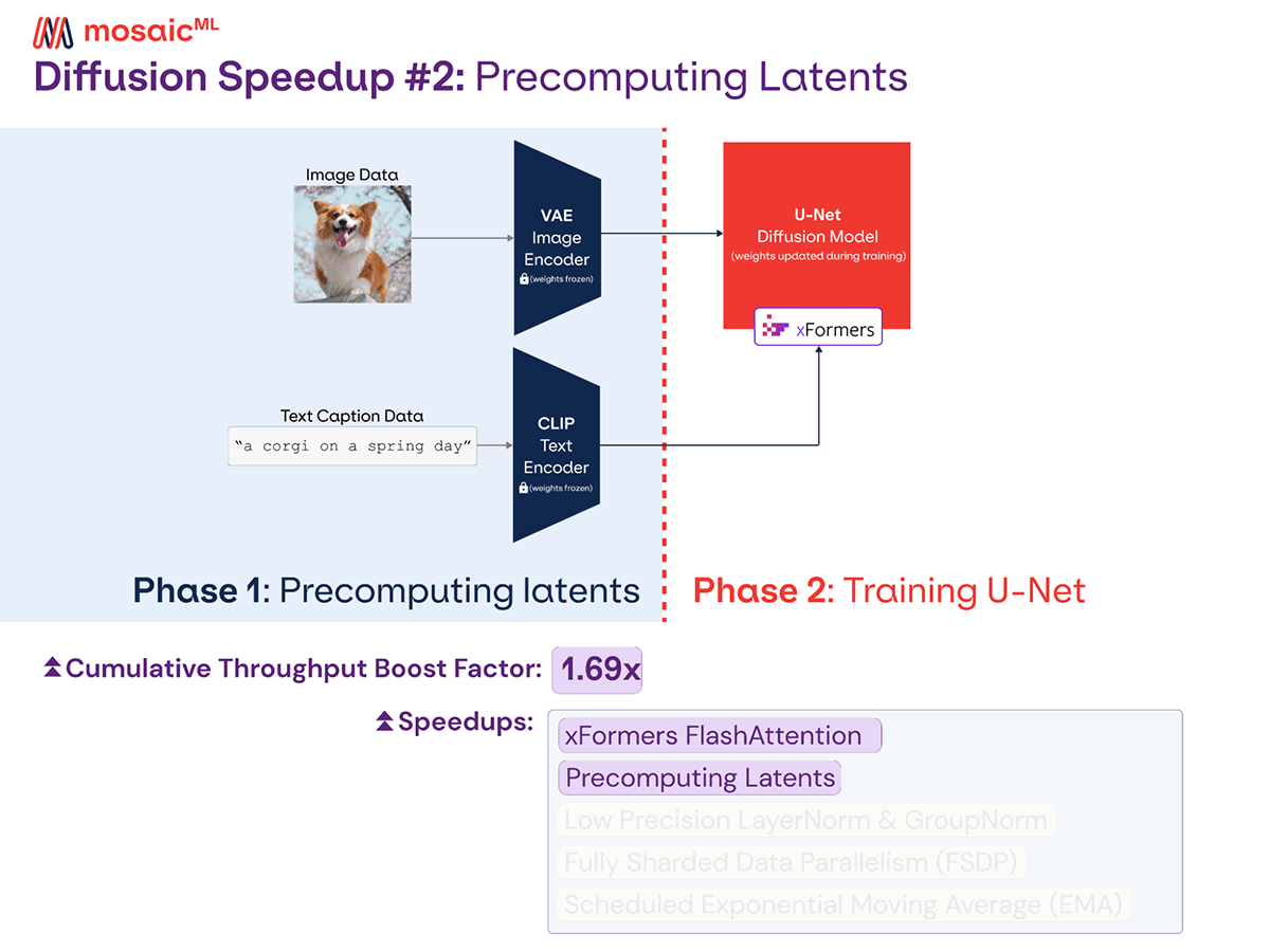
Stable Diffusion is a combination of three models: a variational autoencoder (VAE), a text encoder (CLIP), and a U-Net. During diffusion training, only the U-Net is trained, and the other two models are used to compute the latent encodings of the image and text inputs. Standard training involves computing the VAE and CLIP latents for every batch, but this does a lot of duplicate work when training for multiple epochs: latents are re-computed for each image every time it is used. Instead, we precompute the latents once before training. Empirically, we have 2 epochs at 256 resolution and 5 epochs at 512 resolution, so we avoid 6 extra VAE and CLIP calls per image-text pair in the dataset.
Additionally, when pre-computing the latents, we can lower the precision of the VAE and CLIP models to fp16. This could lead to numerical instability if we were training the VAE and CLIP and used this precision for the backward pass. However, since we're only using them for inference, we can safely lower the precision, which increases speed. The extra memory savings also let us use far larger batch sizes and improve hardware utilization during the latent precomputation.
Low Precision Layernorm and Groupnorm
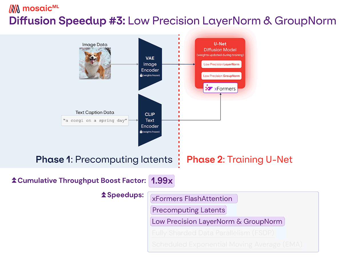
Diffusion training is done in automatic mixed precision by default. This uses half precision (fp16) in most layers, but fp32 in a few numerically unstable layers like normalization and softmax. The Stable Diffusion U-Net architecture uses several LayerNorm and GroupNorm layers, which by default are run in fp32.
Motivated by our finding that half precision LayerNorms are safe to use in language models, we decided to try out half precision LayerNorm and GroupNorm layers. This change resulted in identical loss curves and no instability in our experiments.
While we did observe some throughput improvement, the real benefit was decreased memory usage. Now, along with removing the VAE and CLIP memory by precomputing latents, we have enough space on our 40GB A100 to increase our microbatch size from 8 to 16, 4x larger than what we started with!
Fully Sharded Data Parallelism
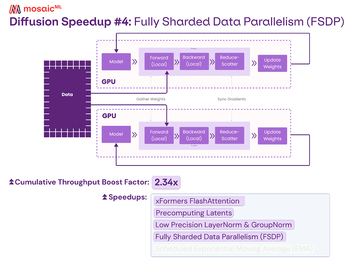
MosaicML Composer, our go-to training library, includes support for PyTorch Fully Sharded Data Parallelism (FSDP). We primarily use this to shard large scale models like 10B+ parameter LLMs that don't fit in a single device across hundreds of GPUs for incredibly fast training. Stable Diffusion doesn't require sharding since it fitsin a single GPU. However, some of the distributed features in FSDP are still useful for speeding up training on a large number of GPUs.
When batches don't fit into memory, we do several forward and backward passes on smaller microbatches, followed by a single gradient update. If we use a small number of GPUs to train, we have far more forward and backward passes per gradient update, so the time spent on the gradient update doesn't matter. However, at 128+ GPUs with a microbatch size of 16, we're only doing one forward and one backward pass for each gradient update. At this scale, the gradient update step starts to become a significant bottleneck.
To tackle this problem, we use FSDP's SHARD_GRAD_OP mode. In normal training, each GPU communicates all its gradients to every other GPU, and then each GPU updates its local copy of the model. With this FSDP variant, each GPU only gets the gradients and updates the weights for a small part of the model before sending the updated weights for that part of the model to all of the other GPUs. By dividing the update step across all the GPUs, we can ensure the amount of work per GPU decreases as we increase the number of GPUs, helping us achieve linear scaling.
Scheduled EMA
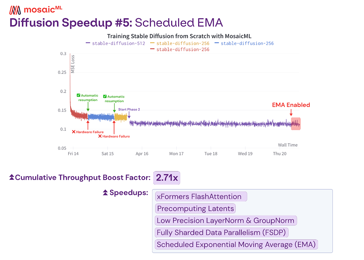
Stable Diffusion 2 uses Exponential Moving Averaging (EMA), which maintains an exponential moving average of the weights. At every time step, the EMA model is updated by taking 0.9999 times the current EMA model plus 0.0001 times the new weights after the latest forward and backward pass. By default, the EMA algorithm is applied after every gradient update for the entire training period. However, this can be slow due to the memory operations required to read and write all the weights at every step.
To avoid this costly procedure, we start with a key observation: since the old weights are decayed by a factor of 0.9999 at every batch, the early iterations of training only contribute minimally to the final average. This means we only need to take the exponential moving average of the final few steps. Concretely, we train for 1,400,000 batches and only apply EMA for the final 50,000 steps, which is about 3.5% of the training period. The weights from the first 1,350,000 iterations decay away by (0.9999)^50000, so their aggregate contribution would have a weight of less than 1% in the final model. Using this technique, we can avoid adding overhead for 96.5% of training and still achieve a nearly equivalent EMA model.
Final Time and Cost Estimates
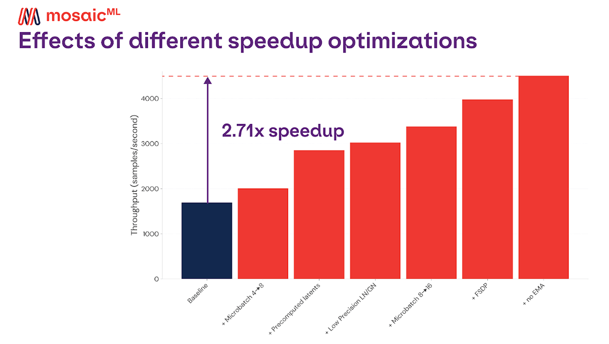
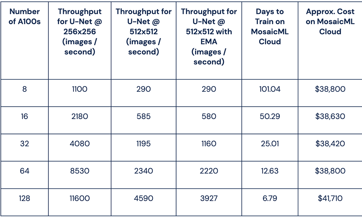
We've shown how we obtained nearly a 3x reduction in time and cost to train Stable Diffusion compared to our original results. With xFormers, precomputed latents, low precision LayerNorm, low precision GroupNorm, FSDP, and scheduled EMA, Table 1 shows it's possible to train Stable Diffusion in just 6.79 days using 21,000 A100-hours for a total cost of less than $42,000. We estimated these times and costs by measuring throughput for training 1.1 billion 256x256 images and 1.7 billion 512x512 images with a max tokenized length of 77 at a global batch size of 2048, as detailed in the Stable Diffusion 2 base model card. This is slightly cheaper than our previously reported run with a cost of $47.7k as it does not account for any time spent on evaluation or restarts due to hardware failures.
These optimizations show that training image generation models from scratch is within reach for everyone. For updates on our latest work, join our Community Slack or follow us on Twitter. If your organization wants to start training diffusion models today, please schedule a demo online or email us at [email protected].
1 When training large models with big batches that don't fit in memory in a single pass, each batch is divided into smaller microbatches. On each device, we can do a forward and backward pass for each microbatch and sum the gradients at the end to compute a gradient update equivalent to a single forward and backward pass with the entire batch all at once.
