Maximizing Equipment Utilization Through Geospatial Analytics
Leveraging Databricks DLT, Spatial Temporal SQL Functions, and H3 for scalable streaming geospatial analytics.
by Tyler Stites, Greg Hansen and Vivian Xie
For working with geospatial data, see this post from Databricks announcing support for Spatial SQL: Introducing Spatial SQL in Databricks: 80+ Functions for High-Performance Geospatial Analytics
Managing high-value equipment deployed across operational sites is a common challenge for construction firms. In response, many original equipment manufacturers are connecting equipment with the Internet of Things, creating new opportunities for digital solutions that drive efficiency across the project lifecycle. According to a 2017 report by McKinsey, technology-driven solutions could improve cross-industry productivity by as much as 60%. Understanding the real-time distribution of equipment can help fleet managers reduce downtime and improve equipment utilization. By leveraging GPS tracking and geospatial analytics, companies can make data-driven decisions about equipment deployment, maintenance scheduling, and resource allocation across work sites.
Delivering real-time results leveraging geospatial data can be difficult and requires complex processing. One common challenge is determining if an asset is operating within a jobsite. Databricks offers the ability to mix several geospatial capabilities together in Delta Live Tables to stream results from point-in-polygon lookups over thousands of sites. Using product APIs for H3 geospatial indexing as well as Spatial Temporal (ST) functions, currently in preview, we can implement the point-in-polygon geospatial “hybrid” join pattern to map equipment locations to specific operational sites with great scalability and accuracy. Once an equipment or fleet manager has a view of each asset’s location, they can calculate statistical insights or reports to help them drive efficient maintenance scheduling, reduce transit and downtime, or dispatch equipment to under-resourced locations.
What is H3?
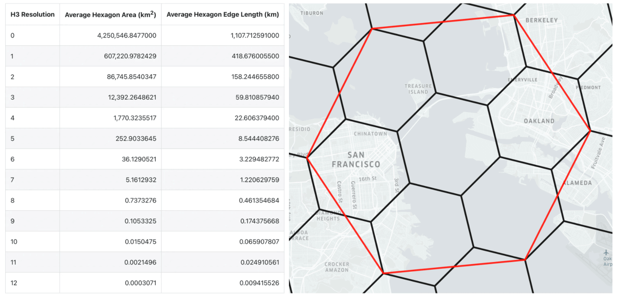
H3 is an open-source geospatial indexing system that divides the Earth into uniform hexagonal cells, each with a unique identifier. Its precision and high scalability makes it ideal for geospatial data analysis.
Key Features of H3:
- Hexagonal Grid System: Uses hexagons instead of squares, ensuring better spatial relationships, minimal distortion, and consistent area coverage.
- Hierarchical Structure: Supports 16 resolutions (0–15), where each level subdivides a hexagon into approximately seven smaller ones, enabling varying precision.
- Efficient Spatial Operations: Simplifies spatial joins, nearest neighbor searches, and point-in-polygon calculations by using cell IDs instead of complex geometries.
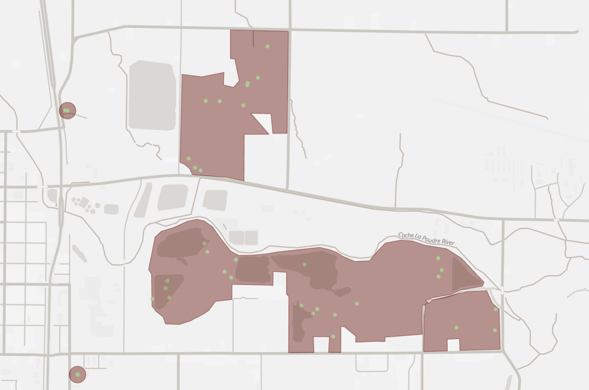
Before we take a look at an example DLT pipeline, let’s visualize our equipment locations and operational site boundaries. The points represent our equipment, the polygons are jobsites, and maintenance sites are circles.
Delta Live Tables Pipeline Overview
This DLT pipeline creates an hourly streaming calculation that shows the percentage of total assets deployed to a jobsite, maintenance site, or in transit between sites. This will allow us to monitor the overall utilization of our equipment fleet.
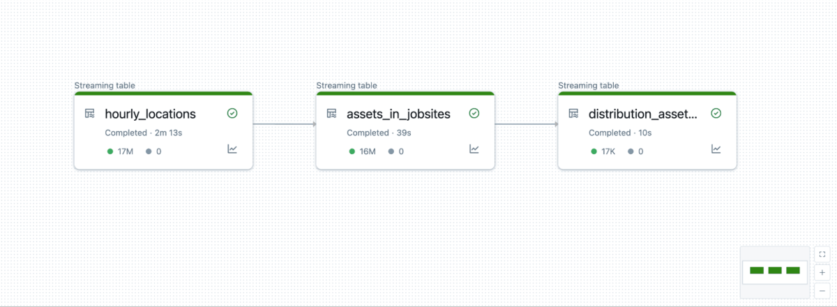
Table 1: Last Hourly Equipment Location
Our first streaming table groups GPS tracking data into hourly windows and selects the last known latitude and longitude position for each piece of equipment.

Table 2: Point-in-Polygon Join with H3 And Spatial Temporal Functions
Now that we have the last location of each asset per hour, we can implement the point-in-polygon join pattern using H3 geospatial indexing to map our assets onto operational sites. In addition, we are using a set of ST functions also provided by Databricks.
Here’s how the code works.
H3 Indexing: Preparing Data for Geospatial Joins
The first step is to assign H3 indices to both the GPS coordinates of assets and the polygon boundaries representing operational sites.
- Resolution Selection: Lower resolutions with larger cells may reduce compute requirements while higher resolutions with smaller cells improve precision. In our example, we chose resolution 11, which is approximately 2,150 square meters and aligns with the level of detail required for our analysis.
Indexing GPS Pointss: Convert the latitude and longitude of each asset's location into an H3 cell ID using h3_longlatash3.
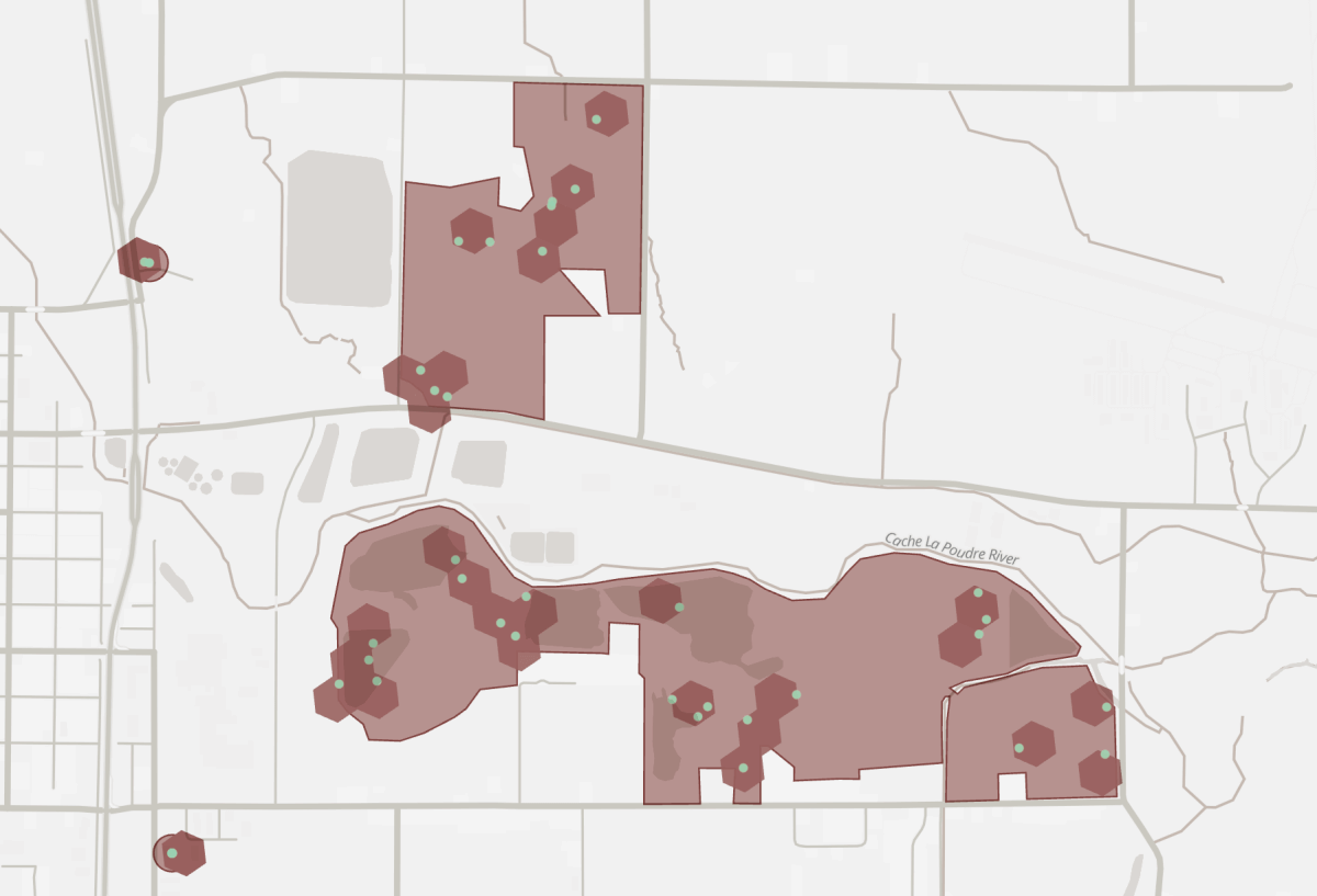
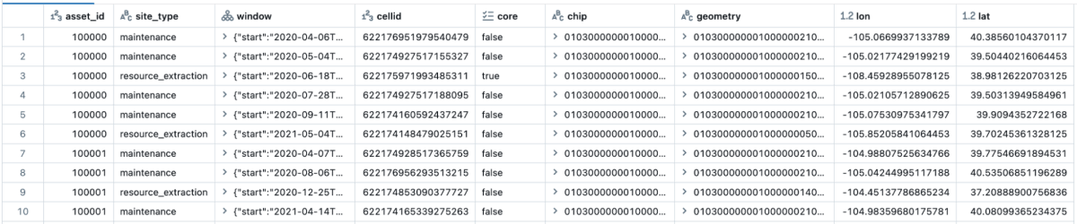
Figure 2: H3 cells assigned to asset locations (dark red hexagon). - Indexing Site Boundaries: Tessellate each site's geometry into the set of H3 cells covering the polygon using h3_tessellateaswkb. This function returns an array with 3 pieces of information:
- “cellid” - H3 cell id(entifier)
- “core” - Categorizes cells as:
- Core = true: Cell is fully contained within the site boundary.
- Core = false (Boundary): Cell is partially overlapping with the site boundary.
“chip” - Geometry representing the intersection or overlap area of the polygon site and H3 Cell.
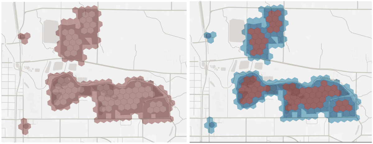
Figure 3: Operational sites tesselated with H3 cells (Left). Tesselated core cells (red) vs boundary cells (blue).
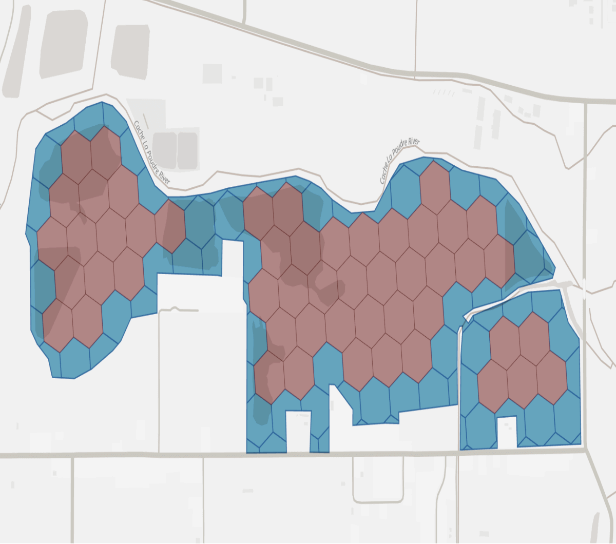
Figure 4: A single site, “Core” H3 cells (red) and site boundary “chips” (blue).
Join Operation: Efficiently Mapping Assets to Sites
The next step is to perform a join operation between the assets and sites based on their H3 cell ID:
- Left Join: Match asset locations with sites using H3 cells.
- Assets located at an operational site.
- Assets at a maintenance site.
- Assets in transit (site_type = null).
- Where: If the “cellid” is a core cell (core = true) we know the cell is fully contained within the site boundary and does not require any further processing.
Joining on H3 cell ID removes the need for running a compute intensive geospatial operation on every record.
Precise Geometric Check for Boundary Cells - The Hybrid Approach
Cells categorized as boundary (core = false) require a precise geometric check because the h3 cell is not completely within the site geometry. We can perform the point-in-polygon check using st_contains. This ensures that only points truly inside the site boundary are included in the join results, eliminating false positives caused by the granularity of the resolution.

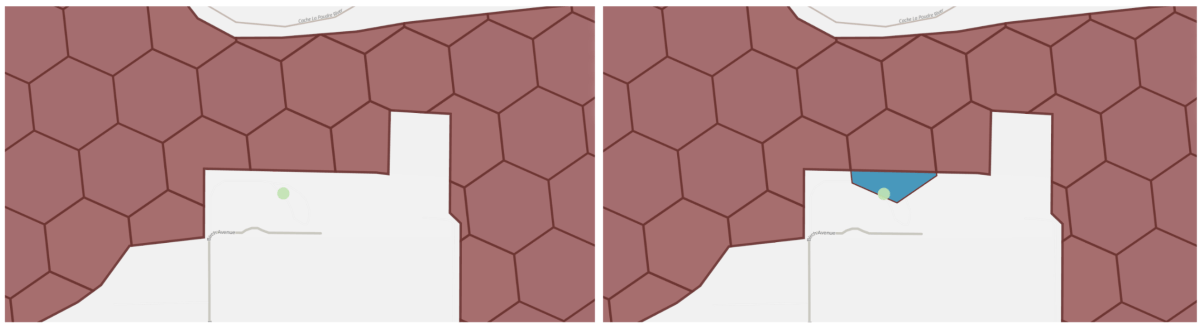
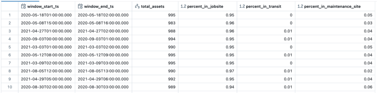
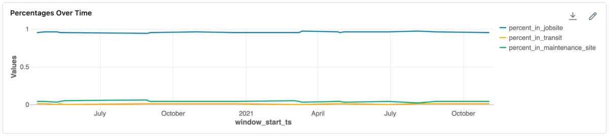
Table 3: Asset Distribution Across Sites
Finally, for the last streaming table in our DLT pipeline, we calculate the distribution of assets across different site types. We use a select expression to count the total number of assets per window, the assets at each site_type, and finally a percentage of the total assets reporting telemetry in each hourly window.
By combining Delta Live Tables with H3 geospatial indexing, Spatial Temporal functions, and the point-in-polygon “hybrid” join pattern, we can efficiently map equipment locations to operational sites and calculate fleet distribution metrics. This approach simplifies spatial operations while maintaining accuracy, making it ideal for real-time geospatial analytics at scale in industries like construction.
Check out our upcoming blogs in this series covering real-time monitoring of landmark entries and exits with stateful streaming and “geospatial agent”, which integrates geospatial intelligence into Databricks Agent framework for real-time delivery tracking.
To learn more about the origins of Geospatial Analytics with H3 on Databricks, check out Spatial Analytics at Any Scale With H3 and Photon. And stay tuned for advancements around Databricks support for ST functions as well as geometry and geography types.
Get the latest posts in your inbox
Subscribe to our blog and get the latest posts delivered to your inbox.