Mitigating Bias in Machine Learning With SHAP and Fairlearn

Try this notebook in Databricks.

With good reason, data science teams increasingly grapple with questions of ethics, bias and unfairness in machine learning applications. Important decisions are now commonly made by models rather than people. Do you qualify for this loan? Are you allowed on this plane? Does this sensor recognize your face as, well, your face? New technology has, in some ways, removed human error, intended or otherwise. Far from solving the problem, however, technology merely reveals a new layer of questions.

It's not even obvious what bias means in a given case. Is it fair if a model recommends higher auto insurance premiums for men, on average? Does it depend on why the model does this? Even this simple question has plausible yet contradictory answers.

If we can't define bias well, we can't remedy it. This blog will examine sources of bias in the machine learning lifecycle, definitions of bias and how to quantify it. These topics are relatively well covered already, but not so much the follow-on question: what can be done about bias once found? So, this will also explore how to apply open source tools like SHAP and Fairlearn to try to mitigate bias in applications.

What is bias?

Most of us may struggle to define bias, but intuitively we feel that "we know it when we see it." Bias has an ethical dimension and is an idea we typically apply to people acting on people. It's not getting a job because of your long hair; it's missing a promotion for not spending time on the golf course.

This idea translates to machine learning models when models substitute for human decision-makers, and typically when these decisions affect people. It feels sensible to describe a model that consistently approves fewer loans for older people as 'biased', but it's odd to call a flawed temperature forecasting model unfair, for example. (Machine learning uses 'bias' as a term of art to mean 'consistent inaccuracy' but that is not its sense here.)

Tackling this problem in machine learning, which is built on formalisms, math, code, and clear definitions, quickly runs into a sea of gray areas. Consider a model that recommends insurance premiums. Which of the following, if true, would suggest the model is fair?

• The model does not use gender as an input
• The model's input includes gender, but analysis shows that the effect of gender on the model's recommended premium is nearly zero
• The average premium recommended for men is the same as that for women
• Among those who caused an accident in the past year, the average premium recommended for men is the same as that for women

Individually, each statement sounds like a plausible criterion, and could match many people's intuition of fairness. They are however materially different statements, and that's the problem. Even if one believes that only one definition is reasonable in this scenario, just imagine a slightly different one. Does the analogous answer suffice if the model were recommending offering a coupon at a grocery store? or recommending release from prison?

Where does bias come from?

Consider a predictive model that decides whether a person in prison will reoffend, perhaps as part of considering whether they qualify for early release. This is the example that this blog will actually consider. Let's say that the model consistently recommends release less frequently for African-American defendants, and that one agrees it is biased. How would this be remediated? Well, where did the bias come from?

Unfortunately, for data science teams, bias does not spring from the machine learning process. For all the talk of "model bias", it's not the models that are unfair. Shannon Vallor (among others) rightly pointed this out when Amazon made headlines for its AI-powered recruiting tool that was reported to be biased against women. In fact, the AI had merely learned to mimic a historically biased hiring process.

"Amazon's system taught itself that male candidates were preferable." No. This is not what happened. Amazon taught their system (with their own hiring data they fed it) that *they* prefer male candidates. This is not a small semantic difference in understanding the problem. https://t.co/Vtv8YUNxW5

— Shannon Vallor (@ShannonVallor) October 10, 2018

The ethical phenomenon of bias comes from humans in the real world. This blog post is not about changing the world, unfortunately.

It's not always humans or society. Sometimes data is biased. Data may be collected less accurately and less completely on some groups of people. All too frequently, headlines report that facial recognition technology underperforms when recognizing faces from racial minority groups. In no small part, the underperformance is due to lack of ethnic or minority representation in the training data. The real faces are fine, but the data collected on some faces is not. This blog will not address bias in data collection, though this is an important topic within the power of technologists to get right.

This leaves the models, who may turn out to be the heroes, rather than villains, of bias in machine learning. Models act as useful summaries of data, and data summarizes the real world, so models can be a lens for detecting bias, and a tool for compensating for it.

How can models help with bias?

Machine learning models are functions that take inputs (perhaps age, gender, income, prior history) and return a prediction (perhaps whether you will commit another crime). If you know that much, you may be asking, "can't we just not include inputs like age, gender, race?". Wouldn't that stop a model from returning predictions that differ along those dimensions?

Unfortunately, no. It's possible for a model's predictions to be systematically different for men versus women even if gender is not an input into the model's training. Demographic factors correlate, sometimes surprisingly, with other inputs. In the insurance premium example, it's possible that "number of previous accidents", which sounds like a fair input for such a model, differs by gender, and thus learning from this value will result in a model whose results look different for men and women.

Maybe that's OK! The model does not explicitly connect gender to the outcome, and if one gender just has more accidents, then maybe it's fine that their recommended premiums are consistently higher.

If bias can be quantified, then model training processes stand a chance of trying to minimize it, just as modeling processes try to minimize errors in their predictions during training. Researchers have adopted many fairness metrics -- equalized odds, equalized opportunity, demographic parity, predictive equality, and so on (see https://fairmlbook.org/classification.html). These definitions generally build on well-understood classification metrics like false positive rate, precision, and recall. Fairness metrics assert that classifier performance, as measured by some metric, is the same across subsets of the data, sliced by sensitive features that "shouldn't" affect the output.

This example considers two commonly-used fairness metrics (later, using the tool Fairlearn): equalized opportunity and equalized odds. Equalized opportunity asserts that recall (true positive rate, TPR) is the same across groups. Equalized odds further asserts that the false positive rate (FPR) is also equal between groups. Further, these conditions assert these equalities conditional on the label. That is to say, in the insurance example above, equalized odds would consider TPR/FPR for men vs women, considering those that had high rates of accidents, separately from those that had none.

These metrics assert "equality of outcome", but do allow for inequality across subsets that were known to have, or not have, the attribute being predicted (perhaps getting in a car accident, or as we'll see, committing a crime again.) That's less drastic than trying to achieve equality regardless of the ground truth.

There's another interesting way in which models can help with bias. They can help quantify the effect of features like age and race on the model's output, using the SHAP library. Once quantified, it's possible to simply subtract those effects. This is an intriguing middle-ground approach that tries to surgically remove unwanted effects from the model's prediction, by explicitly learning them first.

The remainder of this blog will explore how to apply these strategies for remediating bias with open source tools like SHAP, Fairlearn and XGBoost, to a well-publicized problem and dataset: predicting recidivism, and the COMPAS dataset.

Recidivism, and the COMPAS dataset

In 2016, ProPublica analyzed a system called COMPAS. It is used in Broward County, Florida to help decide whether persons in prison should be released or not on parole. based on whether they are predicted to commit another crime (recidivate?). ProPublica claimed to find that the system was unfair. Quoting their report:

• ... black defendants who did not recidivate over a two-year period were nearly twice as likely to be misclassified as higher risk compared to their white counterparts (45 percent vs. 23 percent)
• ... white defendants who re-offended within the next two years were mistakenly labeled low risk almost twice as often as black re-offenders (48 percent vs. 28 percent)

COMPAS uses a predictive model to assign risk decile scores, and there seemed to be clear evidence it was biased against African-Americans. See, for instance, the simple distribution of decile scores that COMPAS assigns to different groups of defendants:

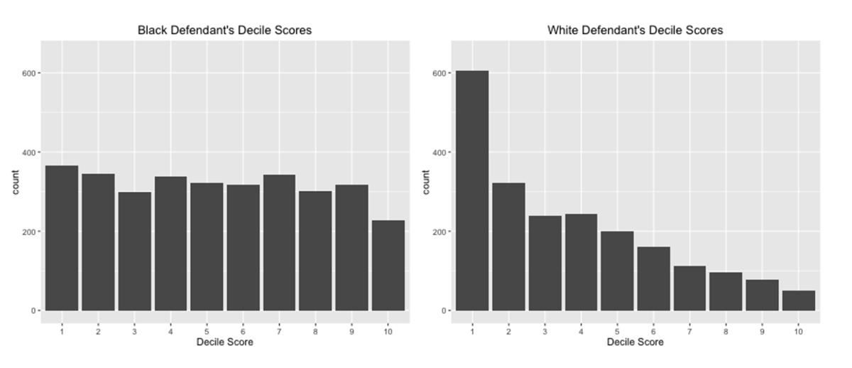
However, whether one judges this system "fair" again depends on how "fairness" is defined. For example, Abe Gong reached a different conclusion using the same data. He argues that there is virtually no difference in the models' outputs between races if one accounts for the observed probability of reoffending. Put more bluntly, historical data collected on released prisoners suggested that African-American defendants actually reoffended at a higher rate compared to other groups, which explains a lot of the racial disparity in model output.

The purpose here is not to analyze COMPAS, the arguments for or against it,or delve into the important question of why the observed difference in rate of reoffending might be so. Instead, imagine that we have built a predictive model like COMPAS to predict recidivism, and now we want to analyze its bias -- and potentially mitigate it.

Thankfully, ProPublica did the hard work of compiling the dataset and cleaning it. The dataset contains information on 11,757 defendants, including their demographics, name and some basic facts about their prior history of arrests. It also indicates whether the person ultimately was arrested again within 2 years, for a violent or non-violent crime. From this data, it's straightforward to build a model.

A first model

It's not necessary to build the best possible model here, merely to build a reasonably good one, in order to analyze the results of the model, and then experiment with modifications to the training process. A simple pass at this might include:

• Turning ProPublica's sqlite DB into CSV files
• Some feature engineering -- ignore defendant name, columns with the same data encoded differently
• Ignore some qualitative responses from the defendant questionnaire in favor of core quantitative facts
• Drop rows missing key data like the label (reoffended or not)
• Fit a simple XGBoost model to it, tuning it with Hyperopt and Spark
• Observe and retrieve the hyperparameter tuning results with MLflow

These choices are debatable, and certainly not the only possible approach. These are not the point of this post, and the details are left to the accompanying notebook. For interest, here is a data profile of this dataset, which is available when reading any data in a Databricks notebook:

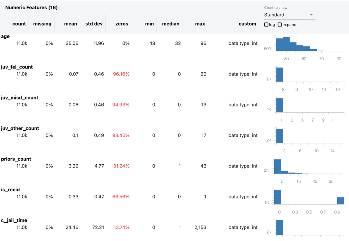
The data set includes demographic information like age, gender and race, in addition to the number of prior convictions, charge degree, and so on. is_recid is the label to predict – did the person recidivate?

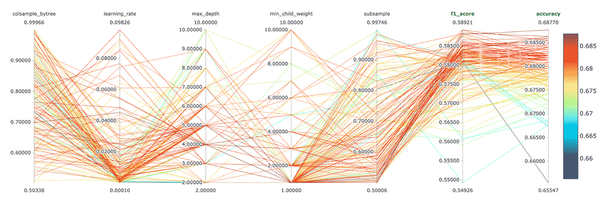
This yields a model with 68.7% accuracy, after a brief hyperparameter search over hundreds of tunings of an XGBoost model with Hyperopt and Spark. The accompanying notebook further uses MLflow to automatically track the models and results; practitioners can re-run and review the tuning results (figure below).

With a trained model in hand, we can begin to assess the training process for evidence of bias in its results. Following the ProPublica study, this example will specifically examine bias that affects African-American defendants. This is not to say that this is the only, or most important, form of bias that could exist.

Attempt 1: Do nothing

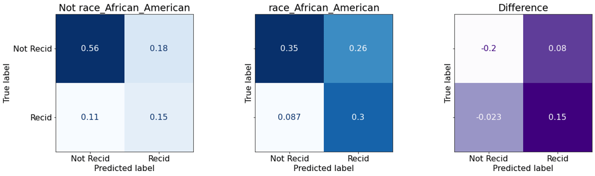
It's useful to first assess fairness metrics on this base model, without any mitigation strategies. The model includes inputs like race, gender and age. This example will focus on equalized odds, which considers true and false positive rates across classes. Standard open source tools can compute these values for us. Microsoft's Fairlearn has utility methods to do so, and with a little matplotlib plotting, we get some useful information out:

def show_confusion_matrix_diff(data_experiment_tag, 
                               drop_cols=[], 
                               race="African_American"):
  recid_df = get_recid_data(data_experiment_tag, drop_cols)
  def get_cm(label):
    data_pd = recid_df[recid_df[f"race_{race}"] == label][["is_recid", "prediction"]]
    return confusion_matrix(data_pd['is_recid'], data_pd['prediction'], 
                            normalize='all')

  not_race_cm = get_cm(0)
  race_cm = get_cm(1)

  _, axes = plt.subplots(1, 3, figsize=(20,5), sharey='row')
  plt.rcParams.update({'font.size': 16})
  labels = ["Not Recid", "Recid"]
  ConfusionMatrixDisplay(not_race_cm, display_labels=labels).\
    plot(ax=axes[0], cmap='Blues', colorbar=False).\
    ax_.set_title(f"Not race_{race}")
  ConfusionMatrixDisplay(race_cm, display_labels=labels).\
    plot(ax=axes[1], cmap='Blues', colorbar=False).\
    ax_.set_title(f"race_{race}")
  ConfusionMatrixDisplay(race_cm - not_race_cm, display_labels=labels).\
    plot(ax=axes[2], cmap='Purples', colorbar=False).\
    ax_.set_title("Difference") 
  plt.show()

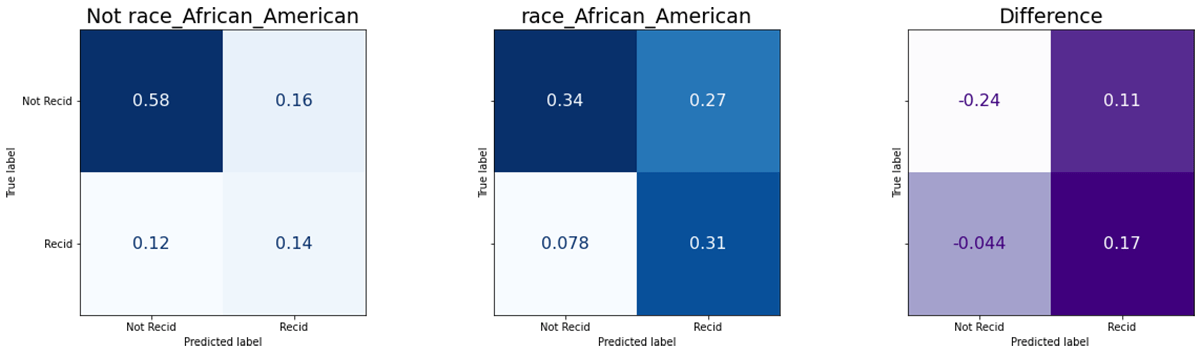
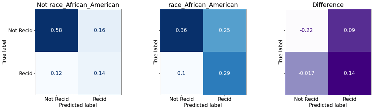
The two blue matrices are confusion matrices, showing classifier performance on non-African-American defendants, and African-American ones. The four values represent the fraction of instances where the classifier correctly predicted that the person would not reoffend (top left) or would reoffend (bottom right). The top right value is the fraction of false positives, and bottom left are false negatives. The purple matrix at the right is simply the difference – rate for African-Americans, minus rate for others.

It's plain that the model makes a positive (will offend) prediction more often for African-American defendants (right columns). That doesn't feel fair, but so far this is just a qualitative assessment. What does equalized odds tell us, if we examine actual TPR/FPR?

def show_fairness_metrics(data_experiment_tag, drop_cols=[]):
  recid_df = get_recid_data(data_experiment_tag, drop_cols)
  metrics = {
    "accuracy": accuracy_score,
    "recall": recall_score,
    "false positive rate": false_positive_rate,
    "false negative rate": false_negative_rate,
    "selection rate": selection_rate
  }
  mf = MetricFrame(metrics=metrics, y_true=y_val, 
                   y_pred=recid_df["prediction"],
                   sensitive_features=X_val["race_African_American"], 
                   control_features=y_val).by_group
  # Update the run with new metrics
  (fpr_not_af_am, fpr_af_am, _, _) = mf['false positive rate']
  (_, _, fnr_not_af_am, fnr_af_am) = mf['false negative rate']
  run_id = find_best_run_id(data_experiment_tag)
  with mlflow.start_run(run_id=run_id):
    mlflow.log_metrics({
      "Not Af-Am FPR": fpr_not_af_am,
      "Af-Am FPR": fpr_af_am,
      "Not Af-Am FNR": fnr_not_af_am,
      "Af-Am FNR": fnr_af_am
    })
  return mf

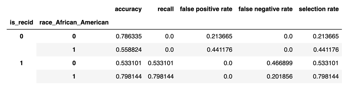
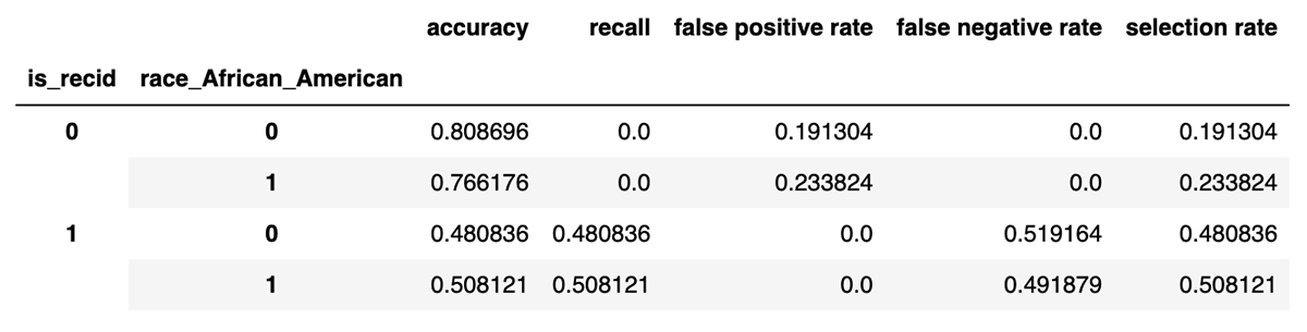
This table has the values that matter for equalized odds. Recall (true positive rate) and false positive rate are broken down by label (did the person actually reoffend later?) and status as African-American or not. There is a difference of 26.5% and 22.8% respectively between African-American and non-African-American defendants. If a measure like equalized odds is the measure of fairness, then this would be 'unfair'. Let's try to do something about it.

Attempt 2: Ignore demographics

What if we just don't tell the model the age, gender or race of the defendants? Is it sufficient? Repeat everything above, merely removing these inputs to the model.

The result is, maybe surprisingly, similar. The gap in TPR and FPR has shrunk somewhat to 19.3% and 18%. This may be counterintuitive. What is the model reasoning about that results in this difference, if it doesn't know race? To answer this, it's useful to turn to SHAP (SHapley Additive Explanations) to explain what the model is doing with all of these inputs:

def draw_summary_plot(data_experiment_tag, drop_cols=[]):
  run_id = find_best_run_id(data_experiment_tag)
  model = mlflow.xgboost.load_model(f"runs:/{run_id}/model")

  train_sample = X_train.drop(drop_cols, axis=1)
  example_samples = np.random.choice(np.arange(len(X_val)), 500, replace=False)
  example = X_val.drop(drop_cols, axis=1).iloc[example_samples]

  explainer = TreeExplainer(model, train_sample, model_output="probability")
  shap_values = explainer.shap_values(example, y=y_val.iloc[example_samples])
  summary_plot(shap_values, example, max_display=10, alpha=0.4, 
               cmap="PiYG", plot_size=(14,6))

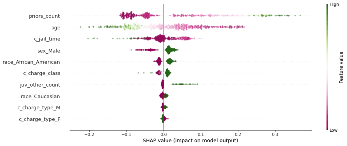
In the above graphic dots represent individual defendants. Rows are features, with more important features shown at the top of the plot. Color represents the value of that feature for that defendant. Green is 'high', so in the first row, green dots are defendants with a high priors_count (number of prior arrests). The horizontal position is SHAP value, or the contribution of that feature for that defendant to the model's prediction. It is in units of the model's output, which is here probability. The right end of the first row shows that the green defendants' high priors_count caused the model to increase its predicted probability of recidivism by about 25-33%. SHAP 'allocates' that much of the final prediction to priors_count.

Being African-American, it seems, has only a modest effect on the model's predictions -- plus a few percent (green dots). Incidentally, so does being Caucasian, to a smaller degree, according to the model. This seems at odds with the observed 'unfairness' according to equalized odds. One possible interpretation is that the model predicts recidivism significantly more often for African-American defendants not because of their race per se, but because on average this group has a higher priors count.

This could quickly spin into a conversation on social justice, so a word of caution here. First, this figure does not claim causal links. It is not correct to read that being a certain race causes more recidivism. It also has nothing to say about why priors count and race may or may not be correlated.

Perhaps more importantly, note that this model purports to predict recidivism, or committing a crime again. The data it learns on really tells us whether the person was arrested again. These are not the same things. We might wonder whether race has a confounding effect on the chance of being arrested as well. It doesn't even require a direct link; are neighborhoods where one race is overrepresented policed more than others?

In this case or others, some might view this SHAP plot as reasonable evidence of fairness. SHAP quantified the effects of demographics and they were quite small. What if that weren't sufficient, and equalized odds is deemed important to achieve? For that, it's necessary to force the model to optimize for it.

Attempt 3: Equalized odds with Fairlearn

Model fitting processes try to optimize a chosen metric. Above, Hyperopt and XGBoost were used to choose a model with the highest accuracy. If equalized odds is also important, the modeling process will have to optimize for that too. Fortunately, Fairlearn has several functions that bolt onto standard modeling tools, changing how they fit, to attempt to steer a model's fairness metrics towards the desired direction.

For the practitioner, Fairlearn has a few options. One set of approaches learns to reweight the inputs to achieve this goal. However, this example will try ThresholdOptimizer, which learns optimal thresholds for declaring a prediction "positive" or "negative". That is, when a model produces probabilities as its output, it's common to declare the prediction "positive" when the probability exceeds 0.5. The threshold need not be 0.5; in fact, it need not be the same threshold for all inputs. ThresholdOptimizer picks different thresholds for different inputs, and in this example would learn different thresholds for the group of African-American defendants versus other groups.

def predict_xgboost_fairlearn(X_train_xgb, y_train_xgb, X_val_xgb, y_val_xgb, params):
  mlflow.xgboost.autolog(disable=True)
  pos_weight = (len(y_train_xgb) / y_train_xgb.sum()) - 1
  # Can't use early stopping
  model = XGBClassifier(use_label_encoder=False, n_jobs=4, n_estimators=200, 
                        random_state=0, scale_pos_weight=pos_weight,
                        max_depth=int(params['max_depth']), 
                        learning_rate=params['learning_rate'], 
                        min_child_weight=params['min_child_weight'], 
                        subsample=params['subsample'], 
                        colsample_bytree=params['colsample_bytree'])
  # Wrap in an optimizer that prioritizes equalized odds while 
  # trying to maintain accuracy
  optimizer = ThresholdOptimizer(estimator=model, constraints="equalized_odds", 
    objective="accuracy_score", predict_method="predict_proba")
  sensitive_cols = ["race_African_American"]
  optimizer.fit(X_train_xgb.drop(sensitive_cols, axis=1), y_train_xgb, 
    sensitive_features=X_train_xgb[sensitive_cols])
  wrapper = FairlearnThresholdWrapper(optimizer, sensitive_cols)
  mlflow.pyfunc.log_model("model", python_model=wrapper)
  return wrapper.predict(None, X_val_xgb)

All along, the accompanying code has been using MLflow to track models and compare them. Note that MLflow is flexible and can log 'custom' models. That's important here, as our model is not simply an XGBoost booster, but a custom combination of several libraries. We can log, evaluate and deploy the model all the same:

class FairlearnThresholdWrapper(mlflow.pyfunc.PythonModel):
  def __init__(self, threshold_optimizer, sensitive_cols):
    self.threshold_optimizer = threshold_optimizer
    self.sensitive_cols = sensitive_cols
    
  def predict(self, context, data):
    return self.threshold_optimizer.predict(
      data.drop(self.sensitive_cols, axis=1), 
      sensitive_features=data[self.sensitive_cols], random_state=42)

Trying to optimize for equalized odds comes at a cost. It's not entirely possible to optimize for it and accuracy at the same time. They will trade off. Fairlearn lets us specify that, all else equal, more accuracy is better where equalized odds is achieved. The result?

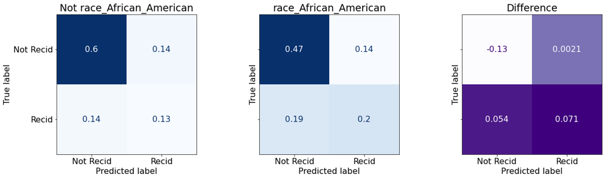
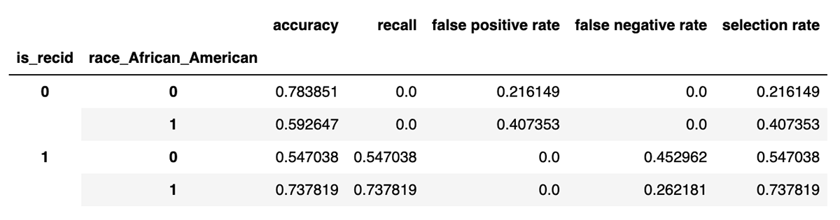
Not surprisingly, the TPR and FPR are much closer now. They're only about 3-4% different. In fact, Fairlearn has a configurable tolerance for mismatch in equalized odds that defaults to 5% -- it's not necessary to demand perfect parity, especially when it may cost accuracy.

Shrinking the TPR/FPR gap did cost something. Generally speaking, the model is more reluctant to classify defendants as "positive" (will recidivate). That means fewer false positives, but more false negatives. Accuracy is significantly lower for those that did reoffend. Whether this is worth the tradeoff is a subjective and fraught question, but tools like this can help achieve a desired point in the tradeoff. Ultimately, the tradeoffs and their tolerance is highly dependent on the application and the ML practitioner thinking about the problem.

This ThresholdOptimizer approach has a problem that returns again to the question of what fairness is. Quite literally, this model has a different bar for people of different races. Some might say that is objectively unfair. Others may argue this is merely counteracting other systematic unfairness, and worth it. Whatever one thinks in this case, the answer could be entirely different in another context!

In cases where this approach may seem unprincipled, there is another possibly more moderate option. Why not simply quantify and then subtract out the demographic effects that were isolated with SHAP?

Attempt 4: Mitigate with SHAP values

Above, SHAP tried to allocate the prediction to each individual input for a prediction. For African-American defendants, SHAP indicated that the model increased its predicted probability of recidivism by 1-2%. Can we leverage this information to remove the effect? The SHAP Explainer can calculate the effect of features like age, race and gender, and sum them, and simply subtract them from the prediction. This can be bottled up in a simple MLflow custom model, so that this idea can be managed and deployed like any other model:

class SHAPCorrectedXGBoostModel(PythonModel):
  
  def __init__(self, booster, explainer, model_columns):
    self.booster = booster
    self.explainer = explainer
    self.sum_shap_indices = 
      [model_columns.tolist().index(c) for c in model_columns if \
       c.startswith("sex") or c.startswith("race")]
    
  def predict(self, context, model_input):
    predicted_probs = self.booster.predict_proba(model_input)[:,1]
    shap_values = self.explainer.shap_values(model_input)
    corrected_probs = predicted_probs - 
      shap_values[:,self.sum_shap_indices].sum(axis=1)
    return pd.DataFrame((corrected_probs >= 0.5).astype('int32'))

It's not so different from the first two results. The TPR and FPR gap remains around 19%. The estimated effect of factors like race has been explicitly removed from the model. There is virtually no direct influence of demographics on the result now. Differences in other factors, like priors_count, across demographic groups might explain the persistence of the disparity.

Is that OK? If it were true that African-American defendants on average had higher priors count, and this legitimately predicted higher recidivism, is it reasonable to just accept that this means African-American defendants are less likely to be released? This is not a data science question, but a question of policy and even ethics.

Finding anomalous cases with SHAP

Time for a bonus round. SHAP's output and plots are interesting by themselves, but they also transform the model inputs into a different space, in a way. In this example, demographics and arrest history turn into units of "contribution predicted probability of recidivism", an alternate lens on the defendants in light of the model's prediction.

Because the SHAP values are in the same units (and useful units at that), they lead to a representation of defendants that is naturally clusterable. This approach differs from clustering defendants based on their attributes, and instead groups defendants according to how the model sees them in the context of recidivism. Clustering is a useful tool for anomaly detection and visualization. It's possible to cluster defendants by SHAP values to get a sense of whether a few defendants are being treated unusually by the model. After all, it is one thing to conclude that on average the model's predictions are unbiased. It's not the same as concluding that every prediction is fair!

It's possible that, in some instances, the model is forced to lean heavily on race and gender in order to correctly predict the outcome for a defendant. If an investigator were looking for individual instances of unfairness, it would be reasonable to examine cases where the model tried to predict "will recidivate" for a defendant but could only come up with that answer by allocating a lot of probability to demographic features. These might be instances where the defendant was treated unfairly, possibly on account of race and other factors.

A fuller treatment of this idea deserves its own post, but as an example, here is a clustering of the defendants by SHAP values, using t-SNE to generate a clustering that prioritizes a clear separation in groups:

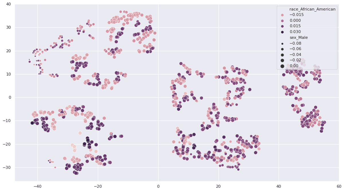
There is some kind of group at the bottom left for which race_African_American caused a different predicted probability of recidivism -- either notably on the high or low side (dark or light points). These are not African-American defendants or not; these are defendants where being or not-being African-American had a wider range of effects. There is a group near the top left for whom gender (sex_Male) had a noticeable negative effect on probability; these are not males, these almost certainly represent female defendants.

This plot takes a moment to even understand, and does not necessarily reveal anything significant in this particular case. It is an example of the kind of exploration that is possible when looking for patterns of bias by looking for patterns of significant effects attributed to demographics.

Conclusion

Fairness, ethics and bias in machine learning are an important topic. What 'bias' means and where it comes from depends heavily on the machine learning problem. Machine learning models can help detect and remediate bias. Open source tools like Fairlearn and SHAP not only turn models into tools for data analysis, but offer means of counteracting bias in model predictions. These techniques can easily be applied to standard open source model training and management frameworks like XGBoost and MLflow. Try them on your model!