
Transformer models, the backbone of modern language AI, rely on the attention mechanism to process context when generating output. During inference, the attention mechanism works by computing the key and value vectors for each token seen so far, and using these vectors to update the internal representation of the next token which will be output. Because the same key and value vectors of the past tokens get reused every time the model outputs a new token, it is standard practice to cache it in a data structure called the Key-Value (KV) cache. Since the KV cache grows proportionally to the number of tokens seen so far, KV cache size is a major factor in determining both the maximum context length (i.e., the maximum number of tokens) and the maximum number of concurrent requests that can be supported for inference on modern language models. Particularly for long inputs, LLM inference can also be dominated by the I/O cost of moving the KV cache from High Bandwidth Memory (HBM) to the GPU’s shared memory. Therefore, decreasing the KV cache size has the potential to be a powerful method to speed up and reduce the cost of inference on modern language models. In this post, we explore ideas recently proposed by Character.AI for reducing KV cache size by replacing most of the layers in the network with sliding window attention (a form of local attention that only uses the key and value vectors of a small number of most recent tokens) and sharing the KV cache amongst layers. We call this architecture MixAttention; our experiments with different variants of this architecture have demonstrated that it maintains both short and long context model quality while improving the inference speed and memory footprint.

We found that KV cache sharing between layers and adding sliding window layers can speed up inference and reduce inference memory usage while maintaining model quality, although some eval metrics show some degradation. In addition, our ablation experiments showed the following:
- Having a few standard attention layers is crucial for the model’s long context abilities. In particular, having the standard KV cache computed in the deeper layers is more important for long context abilities than the standard KV cache of the first few layers.
- KV cache of standard attention layers can be shared between non-consecutive layers without any observed degradation in long context abilities.
- Increasing the KV-cache sharing between sliding window layers too much also hurts long context abilities.
We have provided a guide to configuring and training MixAttention models using LLM Foundry in the appendix of this blog post.
MixAttention Architecture Overview
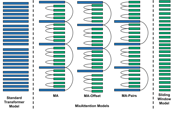
Standard transformer models use global attention in each layer. To create inference-friendly model architectures, we used a combination of sliding window attention layers, standard attention, and KV cache reuse layers. Below is a brief discussion of each component:
- Sliding Window Attention Layers: In Sliding Window Attention (or Local Attention) with window size s, the query only pays attention to the last s keys instead of all the keys preceding it. This means that during inference, the KV cache size needs to only store the KV tensors for the past s tokens instead of storing the KV tensors for all the preceding tokens. In our experiments, we set a window size of s=1024 tokens.
- Standard Attention Layers: We found that even though Standard Attention Layers lead to bigger KV caches and slower attention computation compared to Sliding Window Attention, having a few Standard Attention Layers is crucial for the model’s long context abilities.
- KV cache reuse: This refers to a layer in the transformer network that is reusing the KV cache computed by a previous layer. Hence, if every l layers share KV tensors, then the size of KV cache is reduced by factor of 1/l.
We experimented with different combinations of the components above to ablate the effects of each of them. (Additional combinations are described in the appendices.) We found that not only do each of the above components play important roles in long context abilities and inference speed and memory consumption, but also their relative positions and counts have significant effects on those metrics.
The models we trained are 24-layer Mixture of Experts (MoE) models with 1.64B active and 5.21B total parameters. We used RoPE positional embeddings and increased the RoPE base theta as we increased the context length during training. We used Grouped Query Attention with 12 attention heads and 3 KV heads.
Training
We used LLM Foundry to train MixAttention models. Similar to prior work on training long context models, we followed a multi-stage training procedure to impart long context abilities to the models.
- We pretrained the models with a RoPE theta of 0.5M on 101B tokens, where each sequence has been truncated to 4k token length.
- To increase the context length, we then trained the model on 9B tokens from a mix of natural language and code data, where the sequences have been truncated to 32k tokens. We increased the RoPE theta to 8M for this stage. When training at 32k context length, we trained only the attention weights and froze the rest of the network. We found that this delivered better results than full network training.
- Finally, we trained the model on a 32k-length, synthetic, long-context QA dataset.
- To create the dataset, we took natural language documents and chunked them into 1k-token chunks. Each chunk was then fed to a pretrained instruction model and the model was prompted to generate a question-answer pair based on the chunk. Then, we concatenated chunks from different documents together to serve as the “long context.” At the end of this long context, the question-answer pairs for each of the chunks were added. The loss gradients were computed only on the answer parts of these sequences.
- This phase of training was conducted on 500M tokens (this number includes the tokens from the context, questions, and answers). The RoPE theta was kept at 8M for this stage.
Evaluation
The models were evaluated on the Mosaic Evaluation Gauntlet to measure model quality across various metrics including reading comprehension, commonsense reasoning, world knowledge, symbolic problem solving, and language understanding. To evaluate the models’ long context abilities, we used RULER at a context length of 32000 tokens. RULER is a composite benchmark consisting of 13 individual evals of the following types:
- Needle-in-a-haystack (NIAH): These types of evals hide a single or multiple keys and values in a long text, and the model is evaluated on its ability to retrieve the correct value(s) from the long context for a given key(s).
- Variable Tracking (VT): This eval provides the model with a long context containing variable assignment statements, and the model is tasked to figure out which variables have a particular value by the end of all the variable assignments.
- Common and Frequent Word Extraction (CWE and FWE): These tasks ask the model to extract the most common or frequent words from the text.
- Question Answering (QA): Given a long context, the model is asked a question from somewhere in the context and is evaluated on whether it can correctly answer that question.
We used SGLang to deploy our models on 1 NVIDIA H100 GPU to run RULER and get inference speed and memory consumption metrics.
Results
Position and Count of Standard Attention KV Caches
To measure the effect of the position and count of the standard attention KV caches, we tried four variants. All the configurations are variants of the configuration proposed in Character.AI’s blog post.
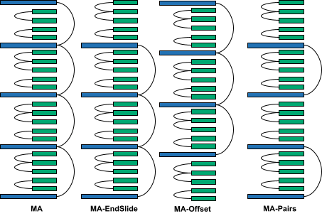
- MA: This variant has a single standard attention KV cache, which is the KV cache of the first layer. All the other standard attention layers share this KV cache.
- MA-EndSlide: This variant is the same as MA, but the last layer is a sliding window attention layer. This was done to measure how much having standard attention in the last layer affects long-context abilities.
- MA-Offset: This variant is similar to MA, but the first standard attention layer is offset to a later layer to allow the model to process the local context for a few layers before the standard attention layer is used to look at longer contexts.
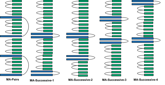
- MA-Pairs: This variant computes two standard attention KV caches (at the first and thirteenth layers), which are then shared with another standard attention layer each.
We compared these models to a transformer model with Standard Attention and a transformer model with Sliding Window Attention in all layers.
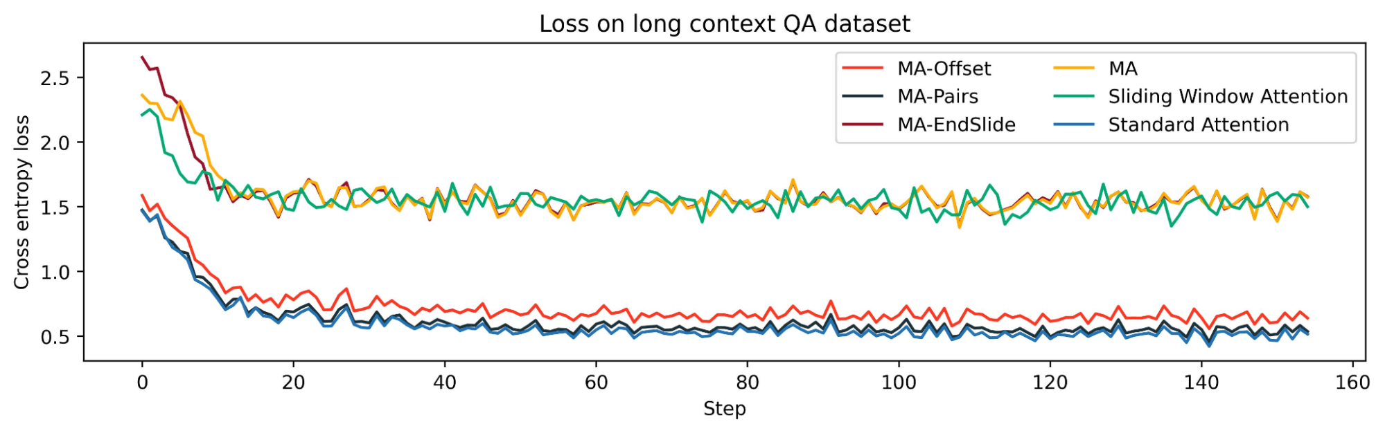

While the loss curves in Stages 1 and 2 of Training were close for all the models, we found that in Stage 3 (training on long context QA dataset), there was a clear bifurcation in the loss curves. In particular, we see that configurations MA and MA-EndSlide show much worse loss than the others. These results are consistent with the long context RULER evals, where we found that MA and MA-EndSlide performed much worse than others. Their performance was similar to the performance of the network with only sliding window attention in all layers. We think the loss in Stage 3 correlates well with RULER evals because unlike Stages 1 and 2, which were next-word prediction tasks where local context was sufficient to predict the next word most of the time, in Stage 3 the model needed to retrieve the correct information from potentially long-distance context to answer the questions.
As we see from the RULER evals, MA-Offset and MA-Pairs have better long-context abilities than MA and MA-EndSlide across all the categories. Both MA and MA-EndSlide have only one standard attention KV cache, which is computed in the first layer, whereas both MA-Offset and MA-Pairs have at least one standard attention KV cache which is computed in deeper layers. Hence, this indicates that having at least one standard attention KV cache computed in the deeper layers of a transformer model is necessary for good long-context abilities.
KV cache sharing in sliding window layers
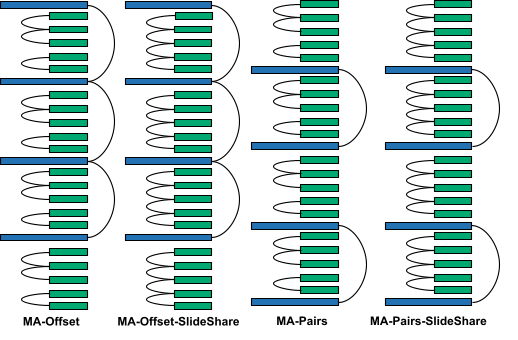
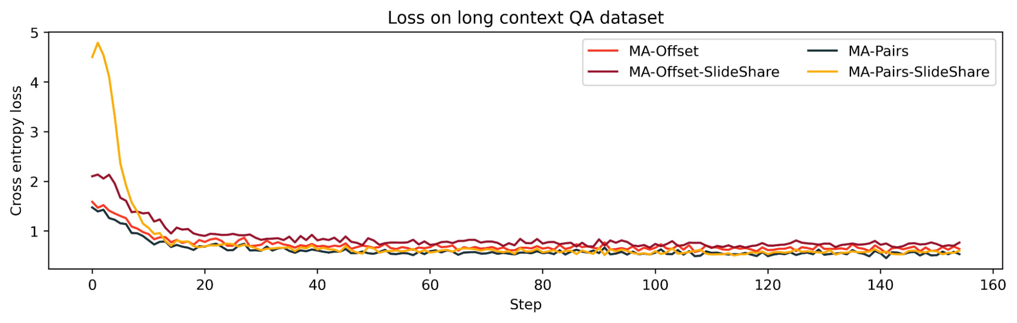
We found that increasing the sharing between sliding window layers degraded the model’s long context performance: MA-Offset-slide-share was worse than MA-Offset and MA-Pairs-SlideShare was worse than MA-Pairs. This shows that the KV cache sharing pattern amongst the sliding window layers is also important for long context abilities.
We have provided the results of some more ablation experiments in the appendices.
Gauntlet Evals
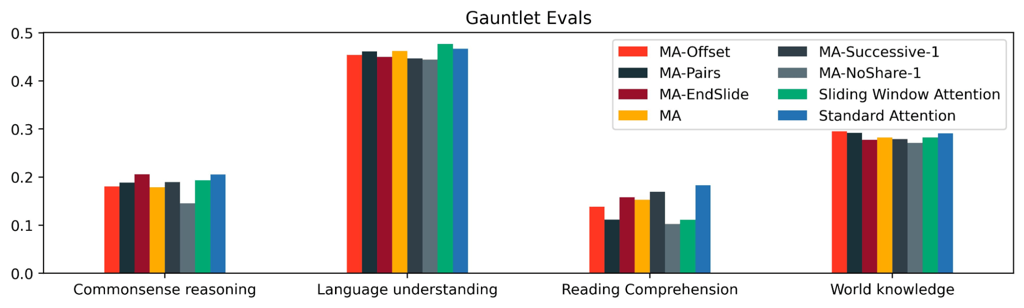
Using the Mosaic Eval Gauntlet v0.3.0, we also measured the performance of MixAttention models on standard tasks like MMLU, HellaSwag, etc. to verify that they retain good shorter context abilities. All of the tasks in this eval suite have context lengths of less than a few thousand tokens.

We found that MixAttention models have similar eval metrics to the baseline model on commonsense reasoning, language understanding, and world knowledge; however, they performed worse on reading comprehension. An interesting open question is if reading comprehension abilities could be improved with a different MixAttention configuration or by training MixAttention models longer.
Inference Speed and Memory Consumption
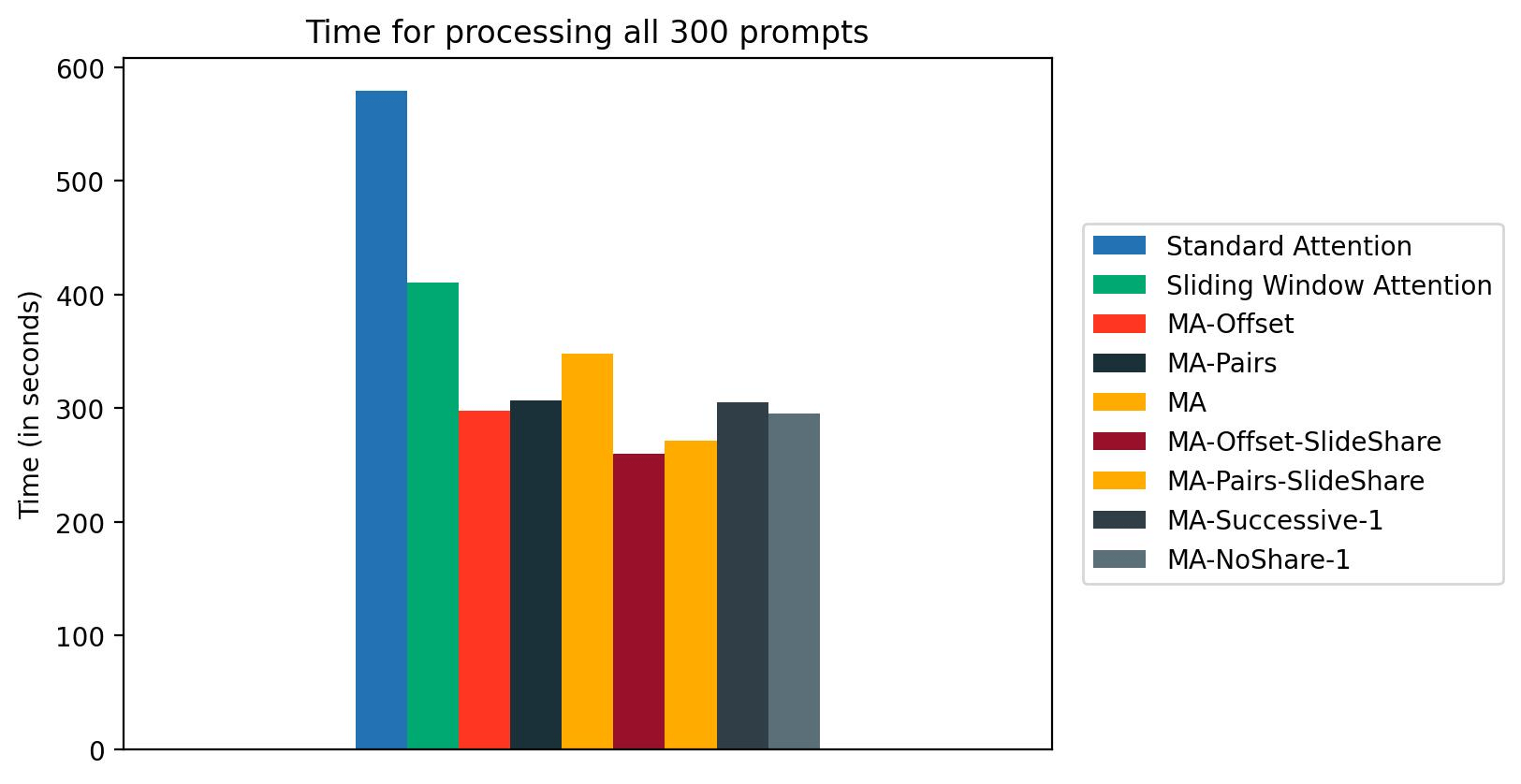
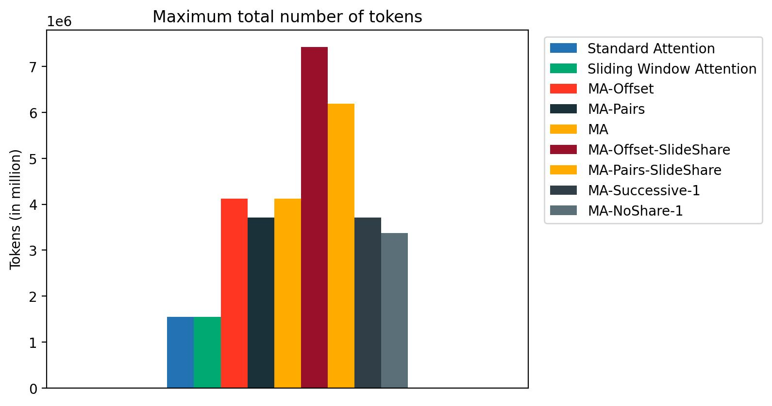
We benchmarked the inference speed and memory consumption of MixAttention models by deploying them on a single NVIDIA H100 GPU using SGLang and querying them with 300 prompts, with an input length of 31000 and output length of 1000. In the figure, we show that the inference speed of MixAttention models is much faster than standard attention models. We also show that with MixAttention, we can support a much larger inference batch size in terms of the total number of tokens.
We found that the current implementation of Sliding Window Attention in SGLang does not optimize the memory consumption for sliding window attention; hence, sliding window attention has the same maximum number of tokens as the standard attention Model. Optimizing the memory consumption for sliding window attention should further increase the maximum number of tokens that MixAttention can support during inference.
Conclusion
We found that MixAttention models are competitive with standard attention models on both long- and short-context abilities while being faster during inference and supporting larger batch sizes. We also observed that on some long context tasks like Variable Tracking and Common Word Extraction, neither MixAttention nor standard attention models performed well. We believe this was because our models weren’t trained long enough or the models need a different kind of long context data to be trained for such tasks. More research needs to be done to measure the impact of MixAttention architectures on those metrics.
We encourage others to explore more MixAttention architectures to learn more about them. Below are a few observations to help with further research:
- Adding a standard attention layer in the initial layers by itself does not seem to help long context abilities (for example, see MA-NoShare-1 in the appendix), even if the KV cache from that layer is reused in layers deeper into the network (MA and MA-EndSlide). Hence we recommend placing the first standard attention layer deeper in the network (like MA-Offset) or having multiple standard attention layers, at least one of which is computed at a deeper layer (like MA-Pairs).
- Sliding window layers also contribute to the model’s long context abilities. Increasing the KV cache sharing amongst the sliding window layers worsened long context abilities (MA-Offset-SlideShare and MA-Pairs-SlideShare). For that reason, we think that the 2-3 sharing pattern in sliding window layers seems to strike a good balance.
- Sharing full attention KV caches between consecutive layers gave mixed results, with slightly worse accuracy on long context QA tasks (see the appendix).
- In our experiments, MA-Offset and MA-Pair showed great speedup and memory savings during inference, while also maintaining long and short context abilities. Hence, MA-Offset and MA-Pairs might be good configurations for further research.
- MixAttention models can be trained with LLM Foundry. Please see the appendix for guidelines.
In general, there is a large hyperparameter space to explore, and we look forward to seeing a variety of new strategies for reducing the cost of inference via combinations of sliding window attention and KV cache reuse.
Appendix: Using LLM Foundry to train MixAttention models
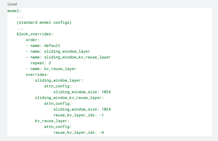
The way to configure MixAttention models with LLM Foundry is to use the block_overrides feature. The block_overrides definition consists of two sections: order and overrides. The order key defines the ordering and the names of the layers in the network, whereas the overrides key contains the custom configuration of each named layer.
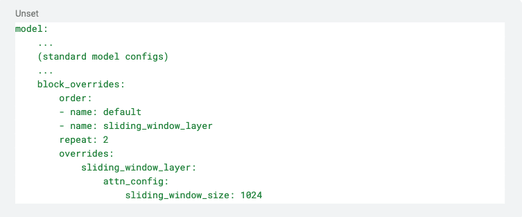
For example, to create a 5 layer network with the first two layers being the standard attention layers, the next two being the sliding window layers, and the last one being a standard attention layer, we use the following YAML:
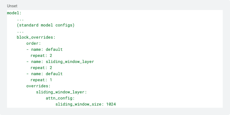
Here, the order section conveys that the first two layers are of type ‘default’, the next two are of type ‘sliding_window_layer’, and the last is of type ‘default’ again. The definitions of each of these types are contained in the overrides section using the names defined in the order section. It says that the ‘sliding_window_layer‘ should have a sliding_window_size of 1024. Note that ‘default’ is a special type, which does not need a definition in the overrides section because it just refers to the default layer (in this case, a standard attention layer). Also, note that ‘sliding_window_layer‘ is just a custom name and can be replaced with any other arbitrary name as long as that name is correspondingly also defined in the overrides section.
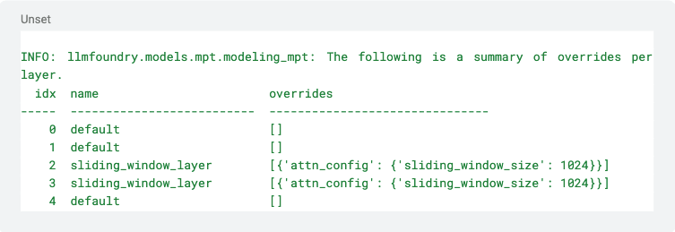
The model configuration is printed in the logs, which can be used to confirm that the model is configured correctly. For example, the above YAML will result in the following being printed in the logs:
We can also configure the two sliding window layers to have different sliding window sizes as follows:
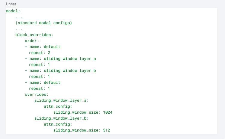
The above will result in the third layer having a sliding window size of 1024, and the fourth layer having a sliding window size of 512. Note that the repeat keyword defaults to 1. So, the above YAML can also be written as:
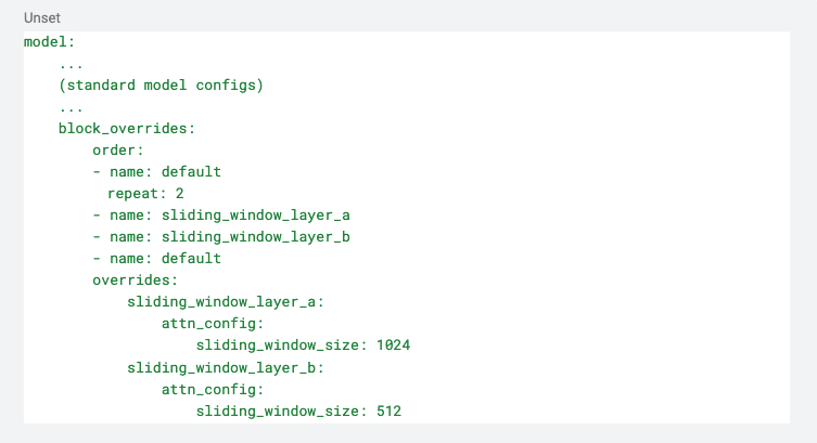
The repeat keyword is also applicable to the order keyword. So, if we want to create a 4 layer network with alternating standard and sliding window attention layers like the following,
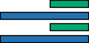
then we can use the following YAML:
To make a layer reuse the KV cache of a previous layer, we use reuse_kv_layer_idx in the attn_config in the override definition. The key reuse_kv_layer_idx contains the relative layer index whose KV cache we want this layer to reuse. To make a two layered network where the second layer reuses the first layer’s KV cache, we can use the following YAML:
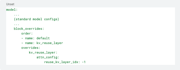
The value -1 indicates that the layer named kv_reuse_layer reuses the KV cache of the layer that is one layer before it. To create a 5 layer network with the following configuration
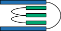
we can use the following YAML:
Note that in the above configuration, layer #4 reuses the KV cache of layer #3, which in turn reuses the KV cache of layer #2. Hence, layer #4 ends up reusing the KV cache of layer #2.
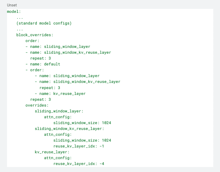
Finally, note that order can be defined recursively; that is, the order can contain another order sub-block. For example, MA-Offset-SlideShare
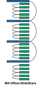
can be defined as follows:
Appendix: Other Ablation Experiments
Sharing Standard Attention KV Caches between Consecutive Layers
Since the transformer layers progressively update the latent representation of a token as it progresses through the layers, the Query, Key, and Value tensors might have significantly different representations for layers that are far apart. Hence, it might make more sense to share KV caches between consecutive layers. To test this, we compared four such configurations: MA-Successive-1, MA-Successive-2, MA-Successive-3, and MA-Successive-4 against MA-Pairs. These configurations vary the positions of the standard KV attention layers and the distance between the consecutive pairs of standard KV attention layers.
Since the transformer layers progressively update the latent representation of a token as it progresses through the layers, the Query, Key, and Value tensors might have significantly different representations for layers that are far apart. Hence, it might make more sense to share KV caches between consecutive layers. To test this, we compared four such configurations: MA-Successive-1, MA-Successive-2, MA-Successive-3, and MA-Successive-4 against MA-Pairs. These configurations vary the positions of the standard KV attention layers and the distance between the consecutive pairs of standard KV attention layers.
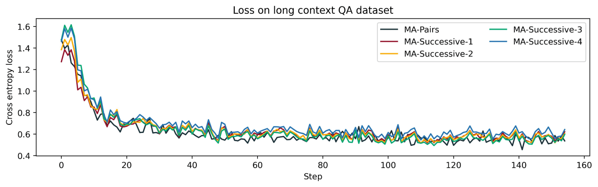
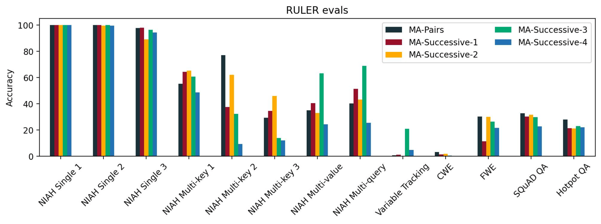
We determined that all the models have similar loss curves and similar performance on NIAH single 1, 2, and 3 tasks, which we consider to be the easiest long context tasks. However, we did not see a consistent pattern across the other NIAH tasks. For long context QA tasks, we found that MA-Pairs was slightly better than the others. These results indicate that sharing standard attention KV cache between layers that are further apart does not lead to any significant degradation in long context abilities as compared to sharing standard attention KV cache between consecutive layers.
Effect of Sharing Standard Attention KV Cache
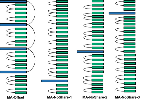
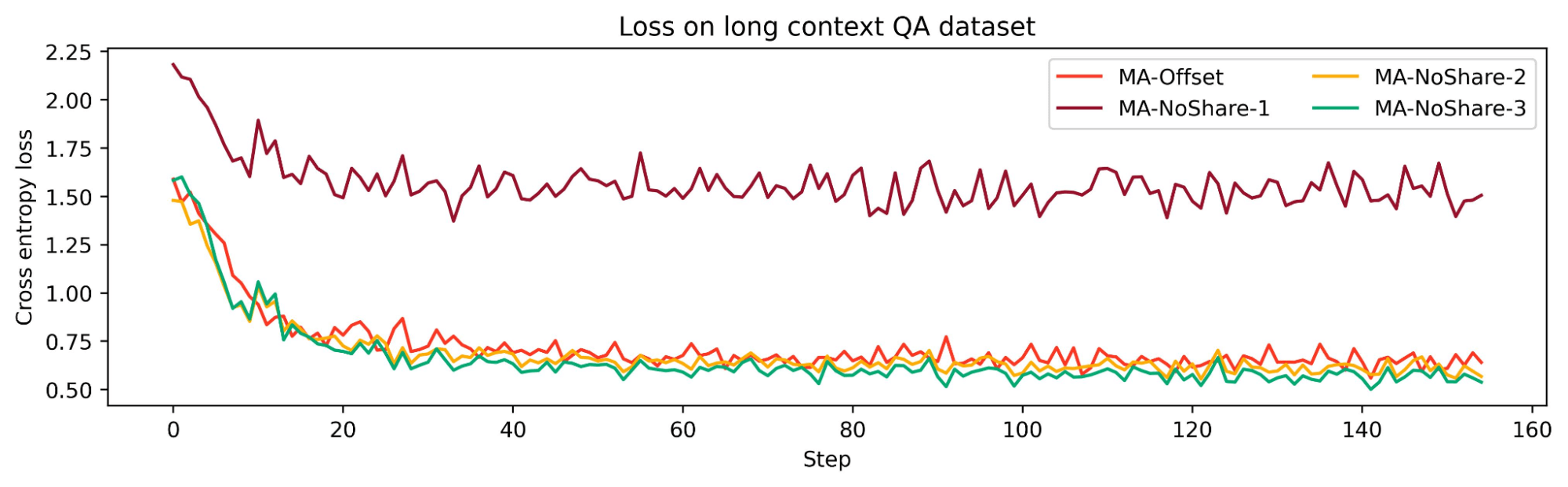
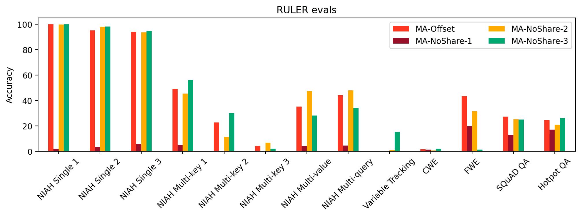
To test the effect of sharing the KV cache between standard attention layers, we tried out three configurations: MA-NoShare-1, MA-NoShare-2, and MA-NoShare-3. We found that MA-NoShare-1 performed very badly on RULER, indicating its lack of long context abilities. However, MA-NoShare-2 and MA-NoShare-3 were comparable to MA-Offset on long context tasks. Hence, we think that further research is needed to ascertain the effects of sharing standard attention KV cache.