Analyzing Apache Access Logs with Databricks
by Ion Stoica and Vida Ha
Databricks provides a powerful platform to process, analyze, and visualize big and small data in one place. In this blog, we will illustrate how to analyze access logs of an Apache HTTP web server using Notebooks. Notebooks allow users to write and run arbitrary Apache Spark code and interactively visualize the results. Currently, notebooks support three languages: Scala, Python, and SQL. In this blog, we will be using Python for illustration.
The analysis presented in this blog and much more is available in Databricks as part of the Databricks Guide. Find this notebook in your Databricks workspace at “databricks_guide/Sample Applications/Log Analysis/Log Analysis in Python” - it will also show you how to create a data frame of access logs with Python using the new Spark SQL 1.3 API. Additionally, there are also Scala & SQL notebooks in the same folder with similar analysis available.
Getting Started
First we need to locate the log file. In this example, we are using synthetically generated logs which are stored in the “/dbguide/sample_log” file. The command below (typed in the notebook) assigns the log file pathname to the DBFS_SAMPLE_LOGS_FOLDER variable, which will be used throughout the rest of this analysis.

Figure 1: Location of the synthetically generated logs in your instance of Databricks Cloud
Parsing the Log File
Each line in the log file corresponds to an Apache web server access request. To parse the log file, we define parse_apache_log_line(), a function that takes a log line as an argument and returns the main fields of the log line. The return type of this function is a PySpark SQL Row object which models the web log access request. For this we use the “re” module which implements regular expression operations. The APACHE_ACCESS_LOG_PATTERN variable contains the regular expression used to match an access log line. In particular, APACHE_ACCESS_LOG_PATTERN matches client IP address (ipAddress) and identity (clientIdentd), user name as defined by HTTP authentication (userId), time when the server has finished processing the request (dateTime), the HTTP command issued by the client, e.g., GET (method), protocol, e.g., HTTP/1.0 (protocol), response code (responseCode), and the size of the response in bytes (contentSize).
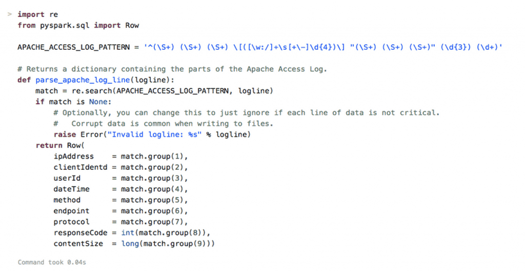
Figure 2: Example function to parse the log file in a Databricks Cloud notebook
Loading the Log File
Now we are ready to load the logs into a Resilient Distributed Dataset (RDD). An RDD is a partitioned collection of tuples (rows), and is the primary data structure in Spark. Once the data is stored in an RDD, we can easily analyze and process it in parallel. To do so, we launch a Spark job that reads and parses each line in the log file using the parse_apache_log_line() function defined earlier, and then creates an RDD, called access_logs. Each tuple in access_logs contains the fields of a corresponding line (request) in the log file, DBFS_SAMPLE_LOGS_FOLDER. Note that once we create the access_logs RDD, we cache it into memory, by invoking the cache() method. This will dramatically speed up subsequent operations we will perform on access_logs.
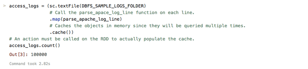
Figure 3: Example code to load the log file in Databricks Cloud notebook
At the end of the above code snippet, notice that we count the number of tuples in access_logs (which returns 100,000 as a result).
Log Analysis
Now we are ready to analyze the logs stored in the access_logs RDD. Below we give two simple examples:
- Computing the average content size
- Computing and plotting the frequency of each response code
1. Average Content Size
We compute the average content size in two steps. First, we create another RDD, content_sizes, that contains only the “contentSize” field from access_logs, and cache this RDD:
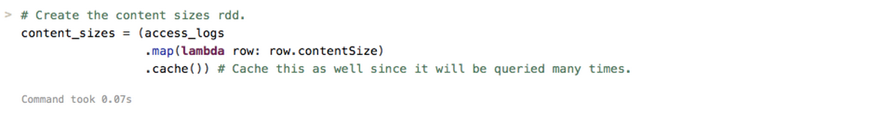
Figure 4: Create the content size RDD in Databricks notebook
Second, we use the reduce() operator to compute the sum of all content sizes and then divide it into the total number of tuples to obtain the average:

Figure 5: Computing the average content size with the reduce() operator
The result is 249 bytes. Similarly we can easily compute the min and max, as well as other statistics of the content size distribution.
An important point to note is that both commands above run in parallel. Each RDD is partitioned across a set of workers, and each operation invoked on an RDD is shipped and executed in parallel at each worker on the corresponding RDD partition. For example the lambda function passed as the argument of reduce() will be executed in parallel at workers on each partition of the content_sizes RDD. This will result in computing the partial sums for each partition. Next, these partial sums are aggregated at the driver to obtain the total sum. The ability to cache RDDs and process them in parallel are the two of the main features of Spark that allows us to perform large scale, sophisticated analysis.
2. Computing and Plotting the Frequency of Each Response Code
We compute these counts using a map-reduce pattern. In particular, the code snippet returns an RDD (response_code_to_count_pair_rdd) of tuples, where each tuple associates a response code with its count.
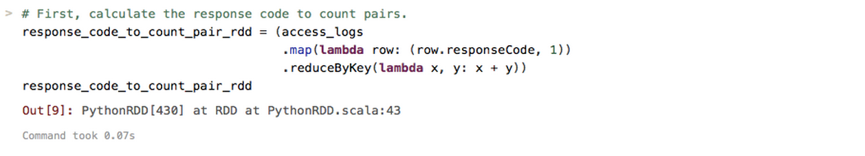
Figure 6: Counting the response codes using a map-reduce pattern
Next, we take the first 100 tuples from response_code_to_count_pair_rdd to filter out possible bad data, and store the result in another RDD, response_code_to_count_array.
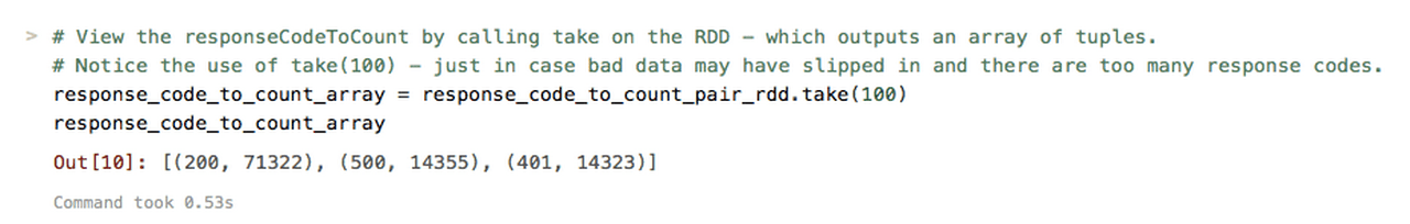
Figure 7: Filter out possible bad data with take()
To plot data we convert the response_code_to_count_array RDD into a DataFrame. A DataFrame is basically a table, and it is very similar to the DataFrame abstraction in the popular Python’s pandas package. The resulting DataFrame (response_code_to_count_data_frame) has two columns “response code” and “count”.
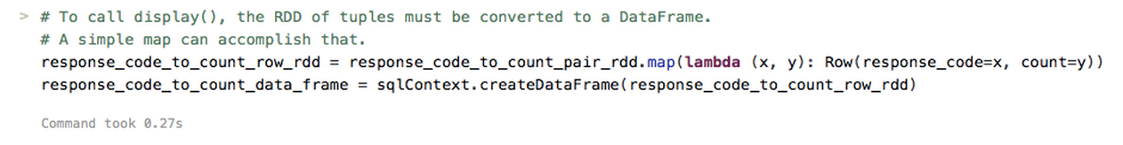
Figure 8: Converting RDD to DataFrame for easy data manipulation and visualization
Now we can plot the count of response codes by simply invoking display() on our data frame.
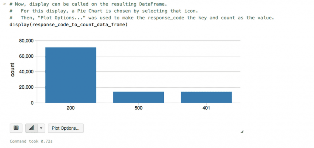
Figure 9: Visualizing response codes with display()
If you want to change the plot size you can do so interactively by just clicking on the down arrow below the plot, and select another plot type. To illustrate this capability, below we show the same data using a pie-chart.
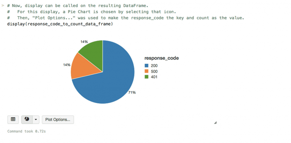
Figure 10: Changing the visualization of response codes to a pie chart
Additional Resources
here.
Other Databricks Cloud how-tos can be found at:
Get the latest posts in your inbox
Subscribe to our blog and get the latest posts delivered to your inbox.