Guest blog: Zen and the Art of Apache Spark Maintenance with Cassandra
This is a guest post from our friends at DataStax.
Apache Cassandra™ is a fully distributed, highly scalable database that allows users to create online applications that are always-on and can process large amounts of data. Apache Spark™ is a processing engine that enables applications in Hadoop clusters to run up to 100X faster in memory, and even 10X faster when running on disk. So it was just a matter of time until the two technologies found each other to deliver ridiculously fast analytics on real-time, operational data stored in a high-performance transactional database.
This blog post will go into details on the inner workings of Spark and how you can shape your application to take advantage of interactions between Spark and Cassandra, and answers to of the most commonly asked questions on the Cassandra + Spark topic.
Spark Architecture Basics
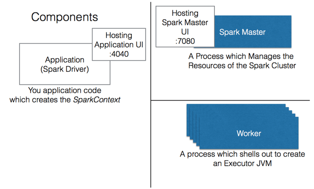
Spark is centered around 4 processes, we can view them on a running system by using the jps command.

Spark Master JVM
Analogous to Hadoop Job Tracker, doesn’t need a lot of RAM since all it does is distribute work to the cluster.
Spark Worker JVM
Analogous to Hadoop Task Tracker, also doesn’t need a lot of RAM since its main responsibility is starting up executor processes.
In DSE/StandAlone mode, a Worker will only start a single executor JVM per application, but this does not mean that you will use only 1 core on the machine. The single executor JVM will use up to the “max cores” set as available on the worker (spark.cores.max). Having more than 1 executor JVM is only possible with multiple workers (a DSE 4.7 feature)
Spark Executor JVM
The most important part of Spark performance. Basically this is going to be a set of processes that do nothing but process RDD tasks.
CPU Requirements
Each core that is allocated to this executor will be able to act on one task at a time. That means a cluster with 20 cores defined by Spark will be able to act on 20 tasks concurrently. If the RDD being processed has less than 20 partitions, then the cluster will not be fully utilized. There will be more details on how tasks/partitions are generated below, but in general the number of tasks should be greater than the number of cores.
You can set more cores available on a worker than there are physical cores. This can have benefits for I/O bound tasks, but it is most likely a bad idea to oversubscribe CPUs on a node also running Cassandra. If oversubscribed, the system will be relying on the OS to decide when Cassandra gets to respond to requests or send out heartbeats. There are some interesting ideas to mitigate this using cgroups to limit cluster resources but I don’t know enough about these strategies to recommend them.
RAM Requirements
Now let’s imagine within this cluster we have 4 physical nodes with 5 cores on each. This means that every machine will have an executor JVM (most likely namedCoarseGrainedExecutorBackend.) This JVM’s heap will be shared between the executors and will have all the same caveats that any other JVM-based application has. A large heap will cause longer garbage collections and extremely large heaps are untenable. The size restriction is of less importance in batch applications like Spark since a 1-second stop the world GC doesn’t mean too much in a 30 minute task. Databricks has a recommended size of 55 GB in the heap. When setting your executor JVM size remember that you are taking away memory from C* and the Operating System. Be sure to leave enough for C* to run and for page cache to help out with C* operations.
RDD Storage Fraction
The largest portion is the cache which will be used for keeping RDD partitions in memory. Since actually retrieving data from Cassandra is most likely going to be a bottleneck for most users since most applications will pull a sizable amount of data from C* and then work on it in memory. The default is 60% of heap and is set with (spark.storage.memoryFraction). Feel free to adjust this but keep in mind the other two portions of the heap. Note: as per the Spark documentation, this fraction should be roughly the same as the old generation size in your JVM.
Application Code and Shuffle Storage
Spark shuffles are organized and performed through a shuffle management service which uses the space in the shuffle.storage portion of the executor to actually move around data (and sort it) before writing it to files and shipping it across the network. Any operations that require a full sort, groupBy, or join will trigger a full shuffle so be careful when reducing this setting (spark.shuffle.memoryFraction) from the default of 0.2. The remaining portion of the heap is for your application code and can be scaled depending on what code and jars are required for your application.
There must be at least the requested amount of RAM available on each worker to create an executor for the Spark Application. In heterogeneous clusters, this means the executor memory can be no larger than the smallest worker if you wish tasks to run on all the machines.
Networking
Among these components the following connections will be established:
- Driver Master
- Master Worker
- Driver Executor
One of the key things to troubleshoot here is the connection between the Driver and the Executors. Usually there is an issue with this communication if jobs start but then terminate prematurely with “unexpected exception in ….” stemming from timed out futures. Most network connectivity issues are because that last link (between the driver and executor) is not successfully being established. Remember that this means that not only must the driver be able to communicate with the executor, but the executor must be able to connect with the driver. If you are having difficulty make sure that the Spark config option spark.driver.host (set in spark-defaults.conf) matches a reachable IP address on the machine running the driver application. In some situations we have found that using an IP address works when having a resolvable domain name does not.
The Anatomy of an RDD
This is where we get real deep real fast. Let’s start about talking about what an RDD is at its very base.
An RDD has several main components:
A Dependency Graph
This details what RDDs must be computed before the current RDD can be successfully executed. This can be empty for an RDD coming from nowhere (like sc.cassandraTable) or a long chain of operations and dependencies (like with rdd.map.filter.shuffle.join.map).
The graph for any RDD can be viewed with toDebugString
Partitions
A description of how the RDD is partitioned and associated metadata describing the properties of each partition. Each partition should be thought of as a discrete chunk of the data represented by the RDD.
Compute Method
A compute method takes a piece of partition metadata (and the task context) and does something to that partition returning an iterator. This is the lazy method which will be executed when an action is called on the RDD.
For example, in the CassandraRDD this method reads metadata for each partition to get Cassandra token ranges and returns an iterator that yields C* data from that range. The Map RDD on the other hand uses the partition to retrieve an iterator from the previous RDD and then applies the given function to that iterator.
Preferred Location Method
A method which describes the preferred location where a particular partition should be computed. This location is defined by the RDD but most RDD types delegate this to the previous RDD in the chain. In all cases, this will be ignored if the partition has been check-pointed since the computed partition already exists. In CassandraRDD this method uses information from the custom partition class to see which node actually contains the ranges specified in the partition. Note that this is a “preferred” not “guaranteed” location. Whether or not a partition will be streamed to another node or computed locally is dependent on the spark.locality.wait parameters. This parameter can be set to 0 to force all partitions to only be computed on local nodes.
When an action is performed on an RDD the dependency tree is analyzed and separated into independent subtrees. Each independent subtree becomes a stage. All of the stages are processed until results can be provided to the user.
Keeping the Dependency Graph Narrow
Many things you do in Spark will only require one partition from the previous RDD (for example: map, flatMap, keyBy). Since computing a new partition in an RDD generated from one of these transforms only requires a single previous partition we can build them quickly and in place. These are the most efficient and reliable operations you can do in Spark. Since each new partition relies only on a single past partition they can be retried independently and should require no network operations.

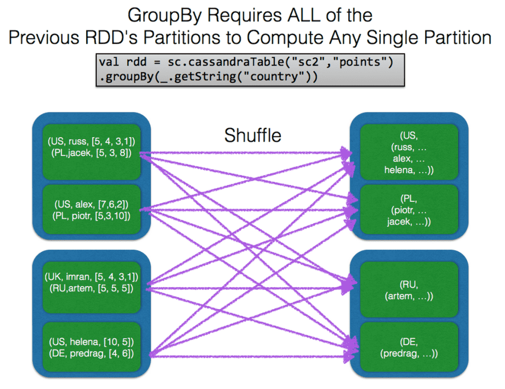
On the other hand some transforms require data being moved about the cluster because they require knowledge of all of the previous RDD’s partitions to work. Transforms such as shuffles, groupBy, join, and sort all require a shuffle under the hood and thus are dependent on all of the previous RDD’s partitions to do their work. You should attempt to keep these transformations to a minimum and push them as far down in your graph as possible (after any filtering you are doing.) It’s also a great idea to cache the result of these expensive actions so that any further references to it will not require a recompute of the entire dependency tree.
Where Operations should be in your Chain of RDD Operations
| Placement | Latest -> | ||||
| Type of Operation | Cassandra RDD Specific | Filters on the Spark Side |
Independent Transforms |
Per Partition Combinable Transforms |
Full Shuffle Operations |
| Examples | where select |
filter sample |
map mapByPartition keyBy |
reduceByKey aggregateByKey |
groupByKey join sort shuffle |
**Note if two RDDs share the same partitioner some of these operations become much cheaper. For example a join between RDDs with the same partitioner is essentially a 1 to 1 partition transform. **
There are several ways to keep your graph narrow and minimize shuffles:
Never let Spark Sort
You almost never *actually* want to sort all your data because every sort has a shuffle and shuffles are not your friend. (What are you going to do with 10 PB of sorted records anyway?) Every shuffle basically erases any data locality you once had as data will be randomly moved throughout your Spark cluster. If the actual goal is a TopX or BottomX consider the top and takeOrdered operations. These operations keep local TopX records on each partition so they don’t require a full shuffle to get the results and locality is preserved. If you need the data to be sorted within subgroup check out the Let Cassandra Sort section below.
One exception to this rule is when writing; there may be occasions when having the data sorted by C* partition key may will allow the Spark Cassandra Connector to write faster. This hasn’t been benchmarked yet and there is bound to be a balance between the time it takes to sort and the amount of data to be written.
Do joins, groupBys, etc. on filtered data sets
The spark dependency graph doesn’t know the internal schema of your data (unless you are using SparkSQL) so that means that spark can’t optimize the execution path. This means the onus is on the developer to ensure that when you eventually do a join or groupBy you use the smallest dataset possible.
This means you want to ensure you never do this:
When you could do this:
Or even better if you are able to push the filter down to Cassandra:
Cache AFTER Hard Work
Any time you have actually done a task which takes a long time (like a shuffle or reading data from C*), that might be a good time to cache your RDD. This tells Spark to make sure that the result of the compute from this RDD is stored. You can specify the storage_level with several parameters; see Spark Programming Guide under RDD Persistence. A cached partition will not have to be recomputed if used multiple times.
Never Collect and then Parallelize: Keep Data On The Cluster
A huge anti-pattern is to collect an RDD, do some work on the driver, then parallelize it back to the cluster. Regardless of which language you are using with Spark, there is no excuse for ever doing work on the driver that could be done on the cluster instead. In practical terms, this means keeping your data as RDDs for the complete duration of the operation. The reason that this is so important is twofold; First, every time you perform a collect you have to serialize the contents of the RDD to the driver application (which may be a small JVM or running on small machine). Second, the client driver isn’t taking advantage of the cluster resources so you are almost guaranteed that driver code will be less performant than similar distributed code.
Example:
Never
Instead:
Take Advantage of Cassandra
The fusion of Spark and Cassandra is more than just availability and durability. Cassandra is a tried a true OLTP solution and we can leverage its advantages within Spark as well!
Let Cassandra Sort
Most of the time if you want your records sorted by some field within a grouping there is no need to have Spark do this work for you. For example, consider a situation where you have incoming scores streaming in for a game which need to be ordered per user. Instead of sorting the data in Spark you can have Cassandra sort the data as it writes it into Cassandra Partitions. This will remove the need for a Spark-side shuffle and it will be quickly retrievable.
Use Cassandra Specific RDD Functions
Remember how I said to be careful with groupBy or Join? Well there are some specific groupBys and joins which are actually very performant and you can (and should) use them as often as you like. These special operations are those which are only acting on data that resides within the same Cassandra partition. Cassandra collocates all data that resides within a Cassandra partition so we won’t need to shuffle and can take advantage of data locality.
Since the raw Spark methods (groupBy, Join) will be shuffling your data, the connector provides new methods which do not require a repartitioning and when doing very specific operations. These methods are spanBy and spanByKey. With these methods you can quickly group up logical rows that share a common primary key without the pain that comes with a shuffle. Once you have grouped your partitions you can perform intra-partition operations on the newly made collections without fear of shuffles.
**Note this functionality currently only works if the span is defined in the clustering key in C*. This means a table with a Primary Key (id, time, type) can be spanned by (id), (id,time), (id,time,type) but not (type) or (time,type). **
Push Down Column Selection
One key way to save on network and serialization costs is to use the select method of the CassandraRDD. This method will push down column selections to Cassandra so the data retrieved and stored in spark is only what you actually want to act on.
For example, instead of:
Use:
Push Down Where Clauses
The Spark Cassandra Connector lets you push down where clauses to the Cassandra database. This will end up letting you do filtering on clustering columns and utilize secondary indexes. Some users may notice that this ends up putting “ALLOW FILTERING” on the underlying Cassandra queries. These same users will most likely be quick to point out that “ALLOW FILTERING” is a known Cassandra smell. This is correct, and you should normally never be using ALLOW FILTERING in a standard Cassandra OLTP application but here we are doing some quite different. In Spark, we won’t be executing these queries very often (hopefully just at RDD generation) and we are already going to hit every node in the cluster from the get go. The major ill effects of secondary indexes revolve around their need to hit all nodes in the cluster and since we are going to be doing this anyway, we can only improve our performance by taking advantage of pushing down this index if it exists. This is especially true as the ratio of “Data That You Want” / “Data In Your Table” shrinks.
RDD/Cassandra Inner joins
When you are already aware of the keys that you want to retrieve from a Cassandra table you can avoid doing a full table scan by using the inner join functionality in the Connector. This functionality is accessed by calling joinWithCassandraTable(keyspace,table) on any RDD writable to Cassandra. This method is most useful when you have a large subset of data from your Cassandra Table which can be specified with partition keys. The additional function repartitionByCassandraReplica(keyspace,table) can be used in cases when the RDD is not already partitioned in a way which is data local with Cassandra. This places all of the requests which will access the same Cassandra node in the same Spark partition.
Worst: Filter on the Spark Side
Bad: Filter on the C* Side in a Single Operation
Best: Filter on the C* side in a distributed and concurrent fashion
Spark Cassandra Connector Metrics
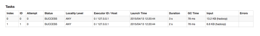
The Spark Cassandra Connector now includes metrics on the throughput to and from Cassandra. These metrics are on by default but can be disabled. They are integrated into the Spark UI so you can now see exactly how many bytes are being serialized to and from Cassandra. To view these metrics go to the stage detail section of the Spark UI and you will see the Input and Output columns populated with the number of bytes read from and written to C*. (Note: Due to the way metrics are implemented in Spark the input and output will be shown as “Hadoop”.)
DataStax at Spark Summit 2015
To learn more about DataStax and our support for Spark, visit our booth at Spark Summit 2015! You can also let us know about what more features you would like in the Spark Cassandra Connector at github.com/datastax/spark-cassandra-connector.
Also, Russ Spitzer, Software Engineer at DataStax, will be sharing his strategies on how to optimize Cassandra and Spark to perform lightning fast analytics on the world’s most scalable OLTP database. This session will be on Monday, June 15th from 4:00 - 4:15pm in Room 1.
Here’s the abstract for more details: https://www.databricks.com/dataaisummit
Never miss a Databricks post
What's next?

Partners
December 11, 2024/15 min read
Introducing Databricks Generative AI Partner Accelerators and RAG Proof of Concepts

News
December 11, 2024/4 min read