New Visualizations for Understanding Apache Spark Streaming Applications
by Tathagata Das, Shixiong Zhu and Andrew Or
Earlier, we presented new visualizations introduced in Apache Spark 1.4.0 to understand the behavior of Spark applications. Continuing the theme, this blog highlights new visualizations introduced specifically for understanding Spark Streaming applications. We have updated the Streaming tab of the Spark UI to show the following:
- Timelines and statistics of events rates, scheduling delays and processing times of past batches.
- Details of all the Spark jobs in each batch.
Additionally, the execution DAG visualization is augmented with the streaming information for understanding the job execution in the context of the streaming operations.
Let’s take a look at these in more detail with an end-to-end example of analyzing a streaming application.
Timelines and Histograms for Processing Trends
When debugging Spark Streaming applications, users are often interested in the rate at which data is being received and the processing time of each batch. The new UI in the streaming tab makes it easy to see the current metrics as well as the trends over that past 1000 batches. While running a streaming application, you will see something like figure 1 below if you visit the streaming tab in the Spark UI (Red letters such as [A] are our annotations, not part of the UI):
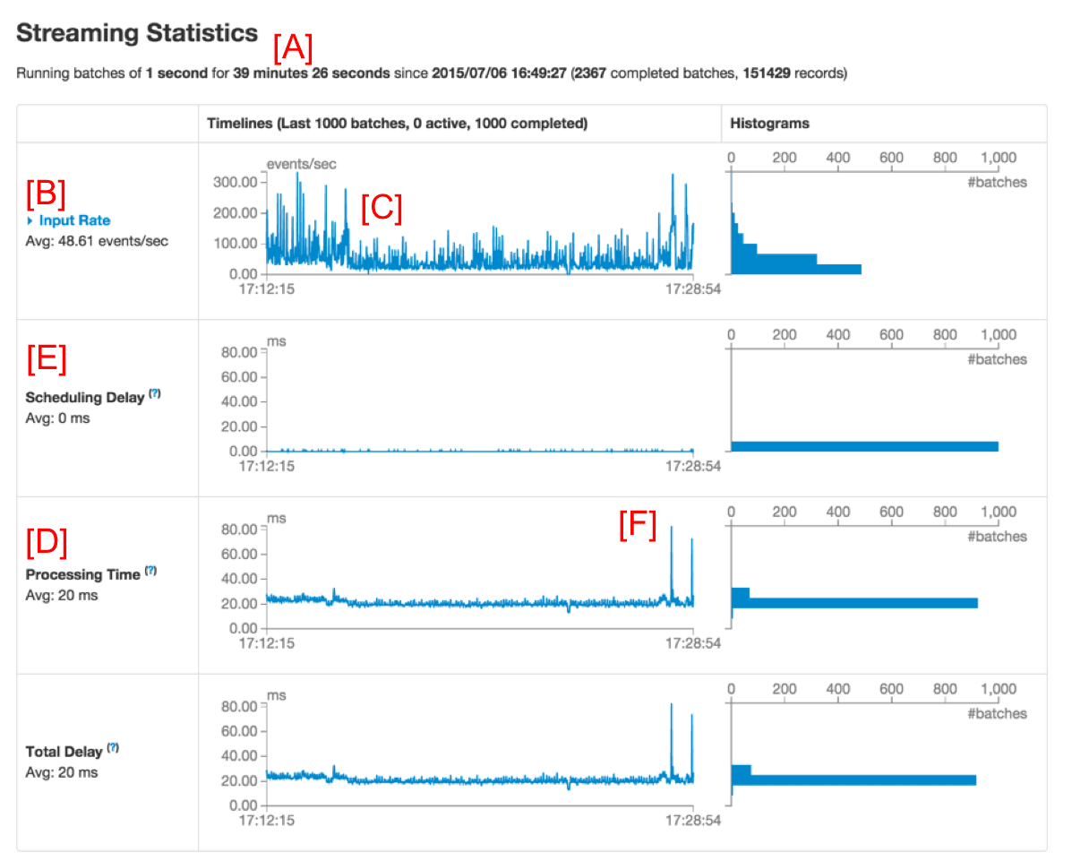
The first line (marked as [A]) shows the current status of the streaming application - in this example, the application has been running for almost 40 minutes at a 1-second batch interval. Below that, the timeline of Input Rate (marked as [B]) shows that the streaming app has been receiving data at a rate of about 49 events/second across all its sources. In this example, the timeline shows a slight dip in the average rate in the middle (marked as [C]), from which the application recovered towards the end of the timeline. If you want get more details, you can click the dropdown beside Input Rate (near [B]) to show timelines organized by each source, as shown in figure 2 below.
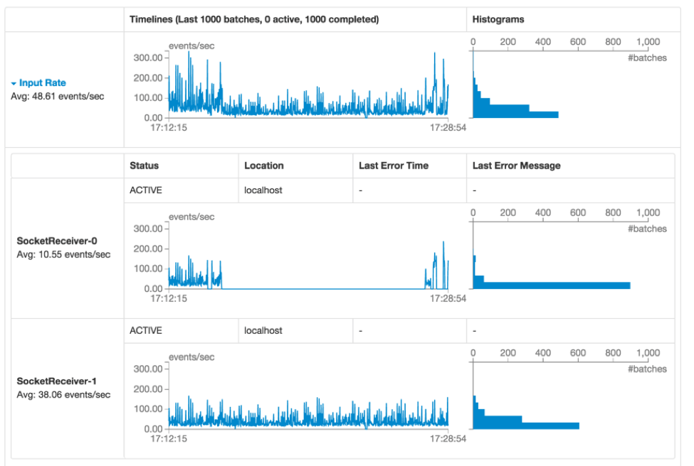
Figure 2 shows that the app had two sources (SocketReceiver-0 and SocketReceiver-1), one of which caused the overall receive rate to dip because it had stopped receiving data for a short duration.
Further down in the page (marked as [D] in figure 1), the timeline for Processing Time shows that these batches have been processed within 20 ms on average. Having a shorter processing time comparing to the batch interval (1s in this example) means that the Scheduling Delay (defined as the time a batch waits for previous batches to complete, and marked as [E] in figure 1) is mostly zero because the batches are processed as fast as they are created. This scheduling delay is the key indicator of whether your streaming application is stable or not, and this UI makes it easy to monitor it.
Batch Details
Referring to figure 1 once again, you may be curious regarding why some batches towards the right took longer to complete (note [F] in figure 1). You can easily analyze this through the UI. First of all, you can click on the points in the timeline graph that have higher batch processing times. This will take you to the list of completed batches further down in the page.
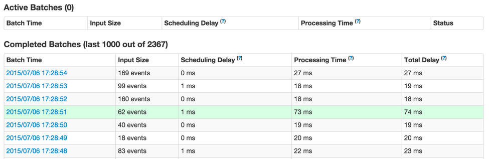
It will show all primary details of the individual batch (highlighted in green in figure 3 above). As you can see, this batch has longer processing time than other batches. The next obvious question is what Spark jobs caused the longer processing time of this batch. You can investigate this by clicking on the batch time (the blue links in the first column), which will take you to the detailed information of the corresponding batch to show you the output operations and their Spark jobs (Figure 4).
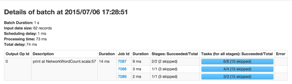
Figure 4 above shows that there was one output operation that generated 3 Spark jobs. You can click on the job IDs to continue digging into the stages and tasks for further analysis.
Execution DAGs of Streaming RDDs
Once you have started analyzing the tasks and stages generated by the batch jobs, it is useful to get a deeper understanding of the execution graph. As shown in the previous blog post, Spark 1.4.0 has added visualizations of the execution DAG (that is, directed acyclic graph) that shows the chain of RDD dependencies and how the RDDs are processed with a chain of dependent stages. If these RDDs are generated by DStreams in a streaming application, then the visualization shows additional streaming semantics. Let’s start with a simple streaming word count program in which we count the words received in each batch. See the example NetworkWordCount. It uses DStream operations flatMap, map and reduceByKey compute the word count. The execution DAG of a Spark job in any batch will look like figure 5 below.
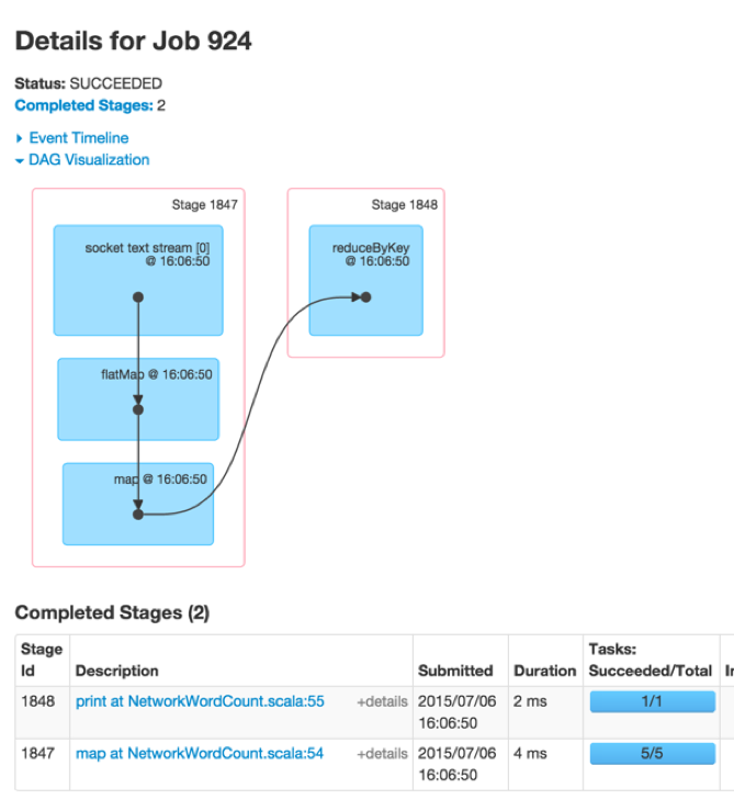
The black dots in the visualization represents the RDDs generated by DStream at batch time 16:06:50. The blue shaded boxes refer to the DStream operations that were used to transform the RDDs, and the pink boxes refer to the stages in which these transformations were executed. Overall this shows the following:
- The data was received from a single socket text stream at batch time 16:06:50
- The job used two stages to compute word counts from the data using the transformations flatMap, map, and reduceByKey.
While this was a simple graph, it can get more complex with more input streams and advanced DStream transformations like window operations and updateStateByKey operation. For example, if we compute counts over a moving window of 3 batches (that is, using reduceByKeyAndWindow) using data from two socket text streams, the execution DAG of one of the batch jobs would look like figure 6 below:
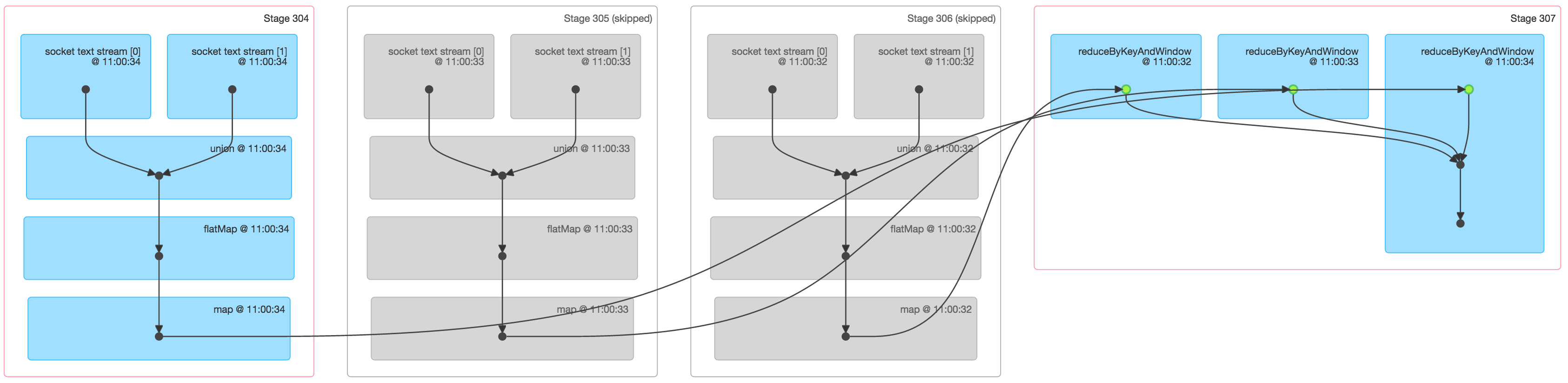
Figure 6 shows a lot of information about a Spark job that counts words across data from 3 batches:
- The first three stages essentially count the words within each of the 3 batches in the window. These are roughly similar to the first stage in the simple NetworkWordCount above, with map and flatMap operations. However note the following differences:
- There were two input RDDs, one from each of the two socket text streams. These two RDDs were unioned together into a single RDD and then further transformed to generate the per-batch intermediate counts.
- Two of these stages are grayed out because the intermediate counts of the older two batches are already cached in memory and hence do not require recomputation. Only the latest batch needs to be computed from scratch.
- The last stage on the right uses reduceByKeyAndWindow to combine per-batch word counts into the “windowed” word counts.
These visualizations enable developers to monitor the status and trends of streaming applications as well as understand their relations with the underlying Spark jobs and execution plans.
Future Directions
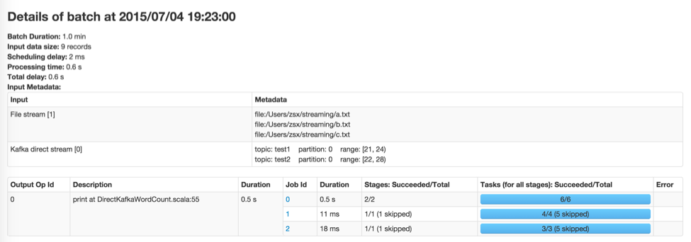
One significant improvement expected in Spark 1.5.0 is more information about input data in every batch (JIRA, PR). For example, if you were using Kafka, the batch details page will show the topics, partitions and offsets processed in that batch. Here is a preview:
Get the latest posts in your inbox
Subscribe to our blog and get the latest posts delivered to your inbox.