rquery: Practical Big Data Transforms for R-Spark Users

This is a guest community blog from Nina Zumel and John Mount, data scientists and consultants at Win-Vector. They share how to use rquery with Apache Spark on Databricks

Introduction

In this blog, we will introduce rquery, a powerful query tool that allows R users to implement powerful data transformations using Apache Spark on Databricks. rquery is based on Edgar F. Codd’s relational algebra, informed by our experiences using SQL and R packages such as dplyr at big data scale.

Data Transformation and Codd's Relational Algebra

rquery is based on an appreciation of Codds' relational algebra. Codd's relational algebra is a formal algebra that describes the semantics of data transformations and queries. Previous, hierarchical, databases required associations to be represented as functions or maps. Codd relaxed this requirement from functions to relations, allowing tables that represent more powerful associations (allowing, for instance, two-way multimaps).

Codd's work allows most significant data transformations to be decomposed into sequences made up from a smaller set of fundamental operations:

• select (row selection)
• project (column selection/aggregation)
• Cartesian product (table joins, row binding, and set difference)
• extend (derived columns, keyword was in Tutorial-D).

One of the earliest and still most common implementation of Codd's algebra is SQL. Formally Codd's algebra assumes that all rows in a table are unique; SQL further relaxes this restriction to allow multisets.

rquery is another realization of the Codd algebra that implements the above operators, some higher-order operators, and emphasizes a right to left pipe notation. This gives the Spark user an additional way to work effectively.

SQL vs pipelines for data transformation

Without a pipe-line based operator notation, the common ways to control Spark include SQL or sequencing SparkR data transforms. rquery is a complementary approach that can be combined with these other methodologies.

One issue with SQL, especially for the novice SQL programmer, is that it can be somewhat unintuitive.

• SQL expresses data transformations as nested function composition
• SQL uses some relational concepts as steps, others as modifiers and predicates.

For example, suppose you have a table of information about irises, and you want to find the species with the widest petal on average. In R the steps would be as follows:

1. Group the table into Species
2. Calculate the mean petal width for each Species
3. Find the widest mean petal width
4. Return the appropriate species

We can do this in R using rqdatatable, an in-memory implementation of rquery:

library(rqdatatable)
## Loading required package: rquery
data(iris)

iris %.>%
  project_nse(., groupby=c('Species'),
              mean_petal_width = mean(Petal.Width)) %.>%
  pick_top_k(.,  
             k = 1,
             orderby = c('mean_petal_width', 'Species'),
             reverse = c('mean_petal_width')) %.>% 
  select_columns(., 'Species')
##      Species
## 1: virginica

Of course, we could also do the same operation using dplyr, another R package with Codd-style operators. rquery has some advantages we will discuss later. In rquery, the original table (iris) is at the beginning of the query, with successive operations applied to the results of the preceding line. To perform the equivalent operation in SQL, you must write down the operation essentially backwards:

SELECT 
   Species 
FROM (
   SELECT 
     Species, 
     mean('Petal.Width') AS mean_petal_width 
   FROM 
     iris
   GROUP BY Species ) tmp1
WHERE mean_petal_width = max(mean_petal_width) /* try to get widest species */
ORDER_BY Species /* To make tiebreaking deterministic */
LIMIT 1     /* Get only one species back (in case of ties) */

In SQL the original table is in the last or inner-most SELECT statement, with successive results nested up from there. In addition, column selection directives are at the beginning of a SELECT statement, while row selection criteria (WHERE, LIMIT) and modifiers (GROUP_BY, ORDER_BY) are at the end of the statement, with the table in between. So the data transformation goes from the inside of the query to the outside, which can be hard to read -- not to mention hard to write.

rquery represents an attempt to make data transformation in a relational database more intuitive by expressing data transformations as a sequential operator pipeline instead of nested queries or functions.

rquery for Spark/R developers

For developers working with Spark and R, rquery offers a number of advantages. First, R developers can run analyses and perform data transformations in Spark using an easier to read (and to write) sequential pipeline notation instead of nested SQL queries. As we mentioned above, dplyr also supplies this capability, but dplyr is not compatible with SparkR -- only with sparklyr. rquery is compatible with both SparkR and sparklyr, as well as with Postgres and other large data stores. In addition, dplyr's lazy evaluation can complicate the running and debugging of large, complex queries (more on this below).

The design of rquery is database-first, meaning it was developed specifically to address issues that arise when working with big data in remote data stores via R. rquery maintains complete separation between the query specification and query execution phases, which allows useful error-checking and some optimization before the query is run. This can be valuable when running complex queries on large volumes of data; you don't want to run a long query only to discover that there was an obvious error on the last step.

rquery checks column names at query specification time to ensure that they are available for use. It also keeps track of which columns from a table are involved with a given query, and proactively issues the appropriate SELECT statements to narrow the tables being manipulated.

This may not seem important on Spark due to its columnar orientation and lazy evaluation semantics, but can be a key on other data store and is critical on Spark if you have to cache intermediate results for any reason (such as attempting to break calculation lineage) and is useful when working traditional row-oriented systems. Also, the effect shows up on even on Spark once we work at scale. This can help speed up queries that involve excessively wide tables where only a few columns are needed. rquery also offers well-formatted textual as well as a graphical presentation of query plans. In addition, you can inspect the generated SQL query before execution.

Example

For our next example let's imagine that we run a food delivery business, and we are interested in what types of cuisines ('Mexican', 'Chinese', etc) our customers prefer. We want to sum up the number of orders of each cuisine type (or restaurant_type) by customer and compute which cuisine appears to be their favorite, based on what they order the most. We also want to see how strong that preference is, based on what fraction of their orders is of their favorite cuisine.

We'll start with a table of orders, which records order id, customer id, and restaurant type.

To work with the data using rquery, we need a rquery handle to the Spark cluster. Since rquery interfaces with many different types of SQL-dialect data stores, it needs an adapter to translate rquery functions into the appropriate SQL dialect. The default handler assumes a DBI-adapted database. Since SparkR is not DBI-adapted, we must define the handler explicitly, using the function rquery::rquery_db_info(). The code for the adapter is here. Let's assume that we have created the handler as db_hdl.

library("rquery")

print(db_hdl) # rquery handle into Spark
## [1] "rquery_db_info(is_dbi=FALSE, SparkR, <environment:>)"
</environment:>

Let's assume that we already have the data in Spark, as order_table. To work with the table in rquery, we must generate a table description, using the function db_td(). A table description is a record of the table's name and columns; db_td() queries the database to get the description.

# assume we have data in spark_handle,
# make available as a view
SparkR::createOrReplaceTempView(spark_handle, "order_table")

# inspect the view for column names
table_description = db_td(db_hdl, "order_table")

print(table_description)
## [1] "table('`order_table`'; custID, restaurant_type, orderID)"
print(column_names(table_description))
## [1] "custID"          "restaurant_type" "orderID"

Now we can compose the necessary processing pipeline (or operator tree), using rquery's Codd-style steps and the pipe notation:

rquery_pipeline %
  extend_nse(., one = 1) %.>%  # a column to help count
  project_nse(., groupby=c("custID", "restaurant_type"),
              total_orders = sum(one)) %.>% # sum orders by type, per customer
  normalize_cols(.,   # normalize the total_order counts
                 "total_orders",
                 partitionby = 'custID') %.>%
  rename_columns(.,  # rename the column
                 c('fraction_of_orders' = 'total_orders')) %.>% 
  pick_top_k(.,  # get the most frequent cuisine type
             k = 1,
             partitionby = 'custID',
             orderby = c('fraction_of_orders', 'restaurant_type'),
             reverse = c('fraction_of_orders')) %.>% 
  rename_columns(., c('favorite_cuisine' = 'restaurant_type')) %.>%
  select_columns(., c('custID', 
                      'favorite_cuisine', 
                      'fraction_of_orders')) %.>%
  orderby(., cols = 'custID')

Before executing the pipeline, you can inspect it, either as text or as a operator diagram (using the package DiagrammeR). This is especially useful for complex queries that involve multiple tables.

rquery_pipeline %.>%
  op_diagram(.) %.>% 
  DiagrammeR::DiagrammeR(diagram = ., type = "grViz")

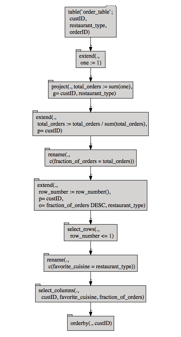
Notice that the normalize_cols and pick_top_k steps were decomposed into more basic Codd operators (for example, the extend and select_rows nodes).

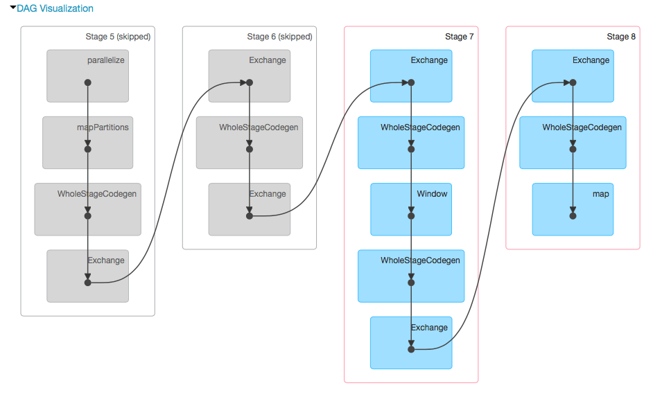
We can also look at Spark’s query plan through the Databricks user interface.

You can also inspect what tables are used in the pipeline, and which columns in those tables are involved.

tables_used(rquery_pipeline)
## [1] "order_table"
columns_used(rquery_pipeline)
## $order_table
## [1] "custID"          "restaurant_type"

If you want, you can inspect the (complex and heavily nested) SQL query that will be executed in the cluster. Notice that the column orderID, which is not involved in this query, is already eliminated in the initial SELECT (tsql_*_0000000000). Winnowing the initial tables down to only the columns used can be a big performance improvement when you are working with excessively wide tables, and using only a few columns.

cat(to_sql(rquery_pipeline, db_hdl))
## SELECT * FROM (
##  SELECT
##   `custID`,
##   `favorite_cuisine`,
##   `fraction_of_orders`
##  FROM (
##   SELECT
##    `custID` AS `custID`,
##    `fraction_of_orders` AS `fraction_of_orders`,
##    `restaurant_type` AS `favorite_cuisine`
##   FROM (
##    SELECT * FROM (
##     SELECT
##      `custID`,
##      `restaurant_type`,
##      `fraction_of_orders`,
##      row_number ( ) OVER (  PARTITION BY `custID` ORDER BY `fraction_of_orders` DESC, `restaurant_type` ) AS `row_number`
##     FROM (
##      SELECT
##       `custID` AS `custID`,
##       `restaurant_type` AS `restaurant_type`,
##       `total_orders` AS `fraction_of_orders`
##      FROM (
##       SELECT
##        `custID`,
##        `restaurant_type`,
##        `total_orders` / sum ( `total_orders` ) OVER (  PARTITION BY `custID` ) AS `total_orders`
##       FROM (
##        SELECT `custID`, `restaurant_type`, sum ( `one` ) AS `total_orders` FROM (
##         SELECT
##          `custID`,
##          `restaurant_type`,
##          1  AS `one`
##         FROM (
##          SELECT
##           `custID`,
##           `restaurant_type`
##          FROM
##           `order_table`
##          ) tsql_80822542854048008991_0000000000
##         ) tsql_80822542854048008991_0000000001
##        GROUP BY
##         `custID`, `restaurant_type`
##        ) tsql_80822542854048008991_0000000002
##      ) tsql_80822542854048008991_0000000003
##      ) tsql_80822542854048008991_0000000004
##    ) tsql_80822542854048008991_0000000005
##    WHERE `row_number` 

Imagine typing in the above SQL. Finally, we can execute the query in the cluster. Note that this same pipeline could also be executed using a sparklyr connection.

execute(db_hdl, rquery_pipeline) %.>%
  knitr::kable(.)

This feature can be quite useful for "rehearsals" of complex data manipulation/analysis processes, where you'd like to develop and debug the data process quickly, using smaller local versions of the relevant data tables before executing them on the remote system.

Conclusion

rquery is a powerful "database first" piped query generator. It includes a number of useful documentation, debugging, and optimization features. It makes working with big data much easier and works with many systems including SparkR, sparklyr, and PostgreSQL, meaning rquery does not usurp your design decisions or choice of platform.

What’s Next

rquery will be adapted to more big data systems allowing R users to work with the tools of their choice. rqdatatable will be extended to be a powerful in-memory system for rehearsing data operations in R.

You can try rquery on Databricks. Simpply follow the links below.

Read More

This example is available as a Databricks Community notebook here and as a (static) RMarkdown workbook here.