Using AutoML Toolkit to Automate Loan Default Predictions
by Benjamin Wilson, Amy Wang and Denny Lee
Download the following notebooks and try the AutoML Toolkit today: Evaluating Risk for Loan Approvals using XGBoost (0.90) | Using AutoML Toolkit to Simplify Loan Risk Analysis XGBoost Model Optimization
This blog was originally published on September 10th, 2019; it has been updated on October 2nd, 2019.
In a previous blog and notebook, Loan Risk Analysis with XGBoost, we explored the different stages of how to build a Machine Learning model to improve the prediction of bad loans. We reviewed three different linear regression models - GLM, GBT, and XGBoost - performing the time-consuming process of manually optimizing the models at each stage.
In this blog post, we will show how you can significantly streamline the process to build, evaluate, and optimize Machine Learning models by using the Databricks Labs AutoML Toolkit. Using the AutoML Toolkit will also allow you to deliver results significantly faster because it allows you to automate the various Machine Learning pipeline stages. As you will observe, we will run the same Loan Risk Analysis dataset using XGBoost 0.90 and see a significant improvement in results with an AUC of 0.6732 to 0.72 using the AutoML Toolkit. In terms of business value (amount of money saved by preventing bad loans), the AutoML Toolkit generated model potentially would have saved $68.88M (vs. $23.22M with the original technique).
What is the problem?
For our current experiment, we will continue to use the public Lending Club Loan Data. It includes all funded loans from 2012 to 2017. Each loan includes applicant information provided by the applicant as well as the current loan status (Current, Late, Fully Paid, etc.) and latest payment information.
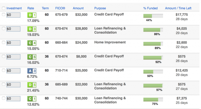
We utilize the applicant information to determine if we can predict if the loan is bad. For more information, refer to Loan Risk Analysis with XGBoost and Databricks Runtime for Machine Learning.
Let’s start with the end
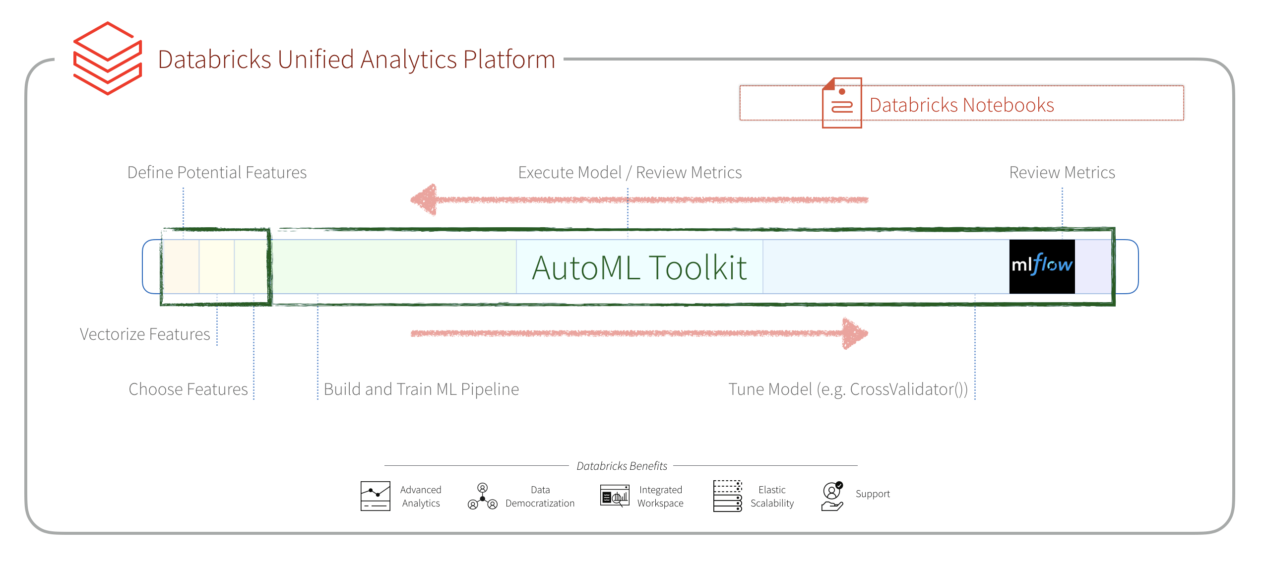
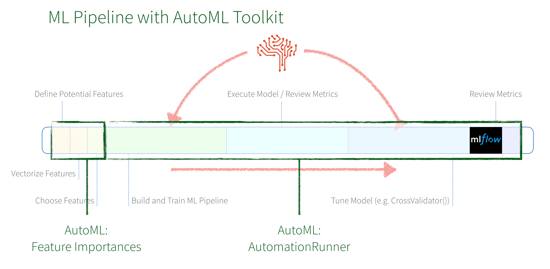
The AutoML Toolkit provides an easy way to automate the various tasks in a Machine Learning Pipeline. In our example, we will use two components: Feature Importances and Automation Runner that will automate the tasks from vectorizing features to iterating and tuning a Machine Learning model.
In brief:
- AutoML’s
FeatureImportancesautomates the discovery of which features (columns from the dataset) are important and should be included when creating a model. - AutoML’s
AutomationRunnerautomates the building, training, execution, and tuning of a Machine Learning pipeline to create an optimal ML model.
When we had manually created a new ML model per Loan Risk Analysis with XGBoost and Databricks Runtime for Machine Learning using XGBoost 0.90, we were able to improve the AUC from 0.6732 to 0.72!
What Did I Miss?
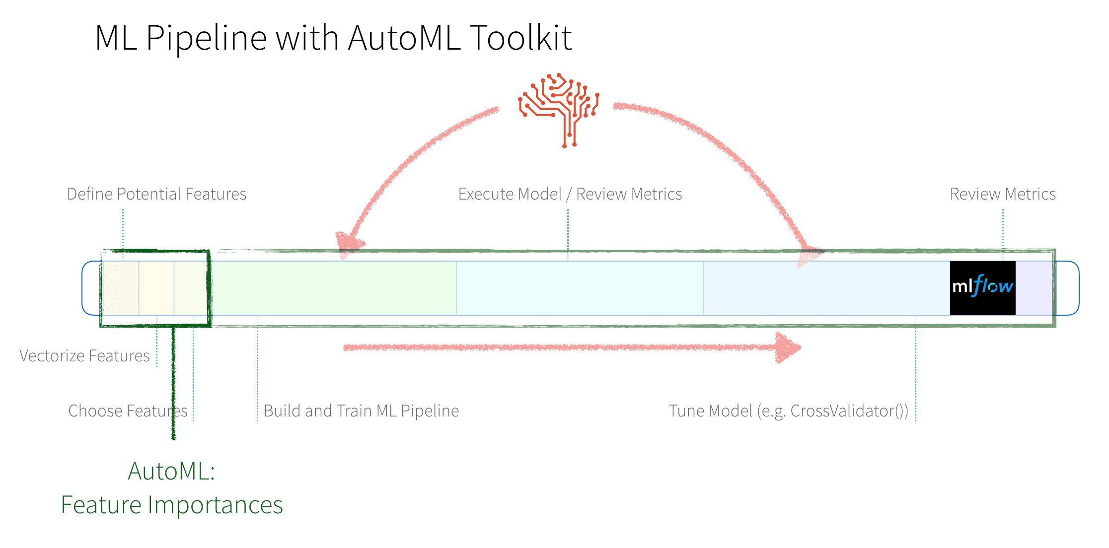
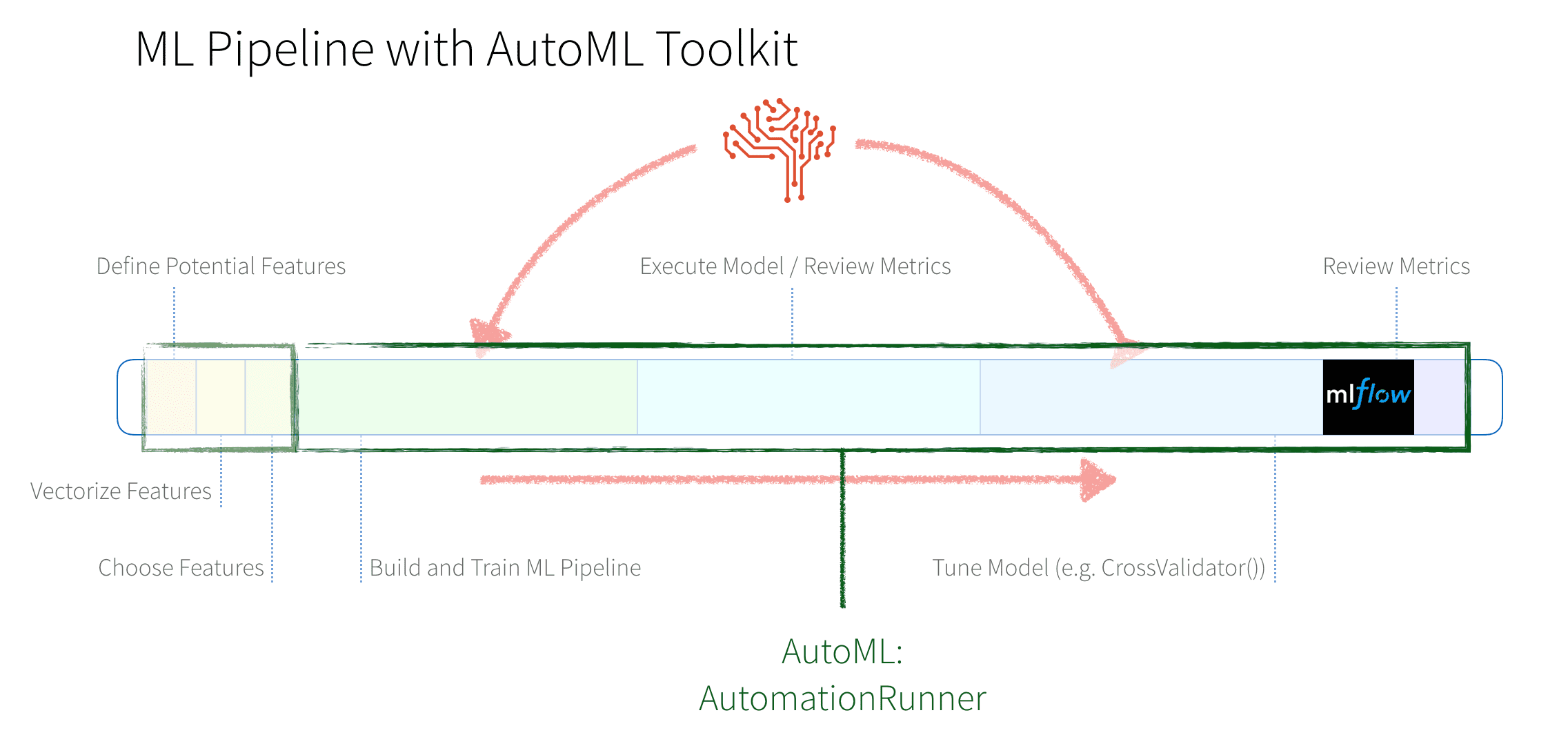
In a traditional ML pipeline, there are many hand-written components to perform the tasks of featurization and model building and tuning. The diagram below provides a graphical representation of these stages.
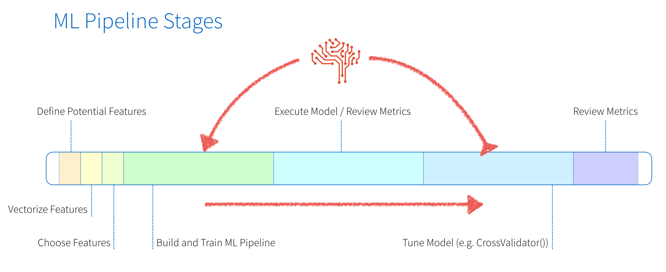
These stages consist of:
- Feature Engineering: We will first define potential features, vectorize them (different steps are required for numeric and categorical data), and then choose the features we will use.
- Model Building and Tuning: These are the highly repetitive stages of building and training our model, executing the model and reviewing the metrics, tuning the model, making changes to the model and repeating this process until finally building our model.
In the next few sections, we will
- Describe with code and visualizations these steps extracted from the Evaluating Risk for Loan Approvals using XGBoost (0.90) notebook
- Show how much simpler this is using the AutoML Toolkit as noted in the Using AutoML Toolkit to Simplify Loan Risk Analysis XGBoost Model Optimization notebook.
Our Feature Presentation
After obtaining reliable and clean data, one of the first steps for a data scientist is to identify which columns (i.e. features) will be used for their model.
Identify Important Features: Traditional ML Pipelines
There are typically a number of steps when choosing which features you will want to use for your model. In our example, we are creating a binary classifier (is this a bad loan or not?) where we will need to define the potential features, vectorize numeric and categorical features, and finally choose the features that will be used in the creation of your model.
Expand to view traditional identifying important features details
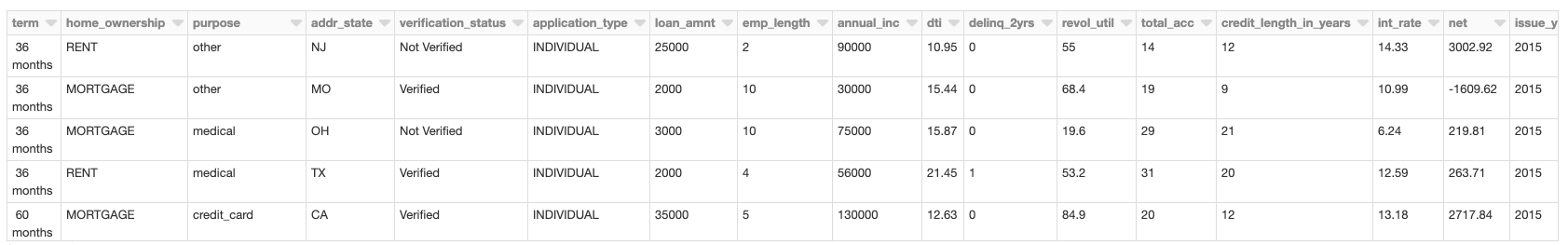
As you can see from the above table, the loan risk analysis dataset contains both numeric and categorical columns. This is an important distinction as there will be a different set of steps for numeric and categorical columns to ultimately assemble a vector that will be used as the input to your ML model.
To better understand if there is a correlation between independent variables, we can quickly examine sourceData using the display command to view this data as a scatterplot.
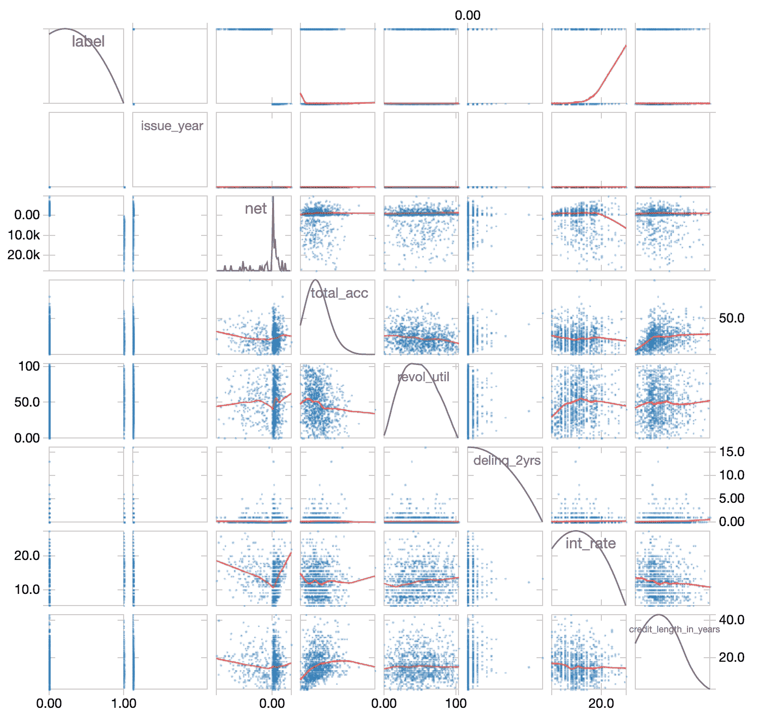
You can further analyze this data by calculating the correlation coefficients; a popular method is to use pandas .corr(). While our Databricks notebook is written in Scala, we can quickly and easily use Python pandas code as noted below.
As noted in the preceding scatterplots (expand above for those details), there are no obvious highly correlated numeric variables. Based on this assessment, we will keep all of the columns when creating the model.
Identifying Important Features: AutoML Toolkit
It is important to note that this process of identifying important features can be a highly iterative and time-consuming process. There are so many different techniques that can be applied, that this process is a book in itself (e.g. Feature Engineering for Machine Learning: Principles and Techniques for Data Scientists).
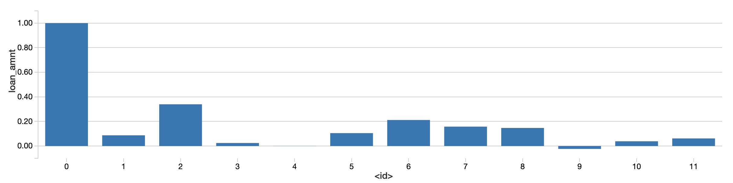
The AutoML Toolkit includes the class FeatureImportances that automatically identifies the most important features; this is all done by the following code snippet.
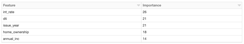
In this specific example, thirty (30) different Spark jobs were automatically generated and executed to find the most important features that need to be included. Note, the number of Spark jobs kicked off will vary depending on several factors. Instead of the days or weeks to manually explore the data, with four lines of code, we identified these features in minutes.
Let’s Build it!
Now that we have identified our most important features, let’s build, train, validate, and tune our ML pipeline for our loan risk dataset.
Traditional Model Building and Tuning
The following steps are an abridged version of Evaluating Risk for Loan Approvals using XGBoost (0.90) notebook code.
Expand to view traditional model building and tuning details
First, we will define our categorical and numeric columns.
Then we will build our ML pipeline as noted by the code snippet below. As noted by the comments in the code, our pipeline has the following steps:
- VectorAssembler: Assemble a features vector based on our feature columns that have been processed by the following
- Inputer estimator for completing missing values for our numeric data
- StringIndexer to encode a string value to a numeric value
- OneHotEncoding to map a categorical feature (represented by the StringIndexer numeric value) to a binary vector
- LabelIndexer: Specify what our label is (i.e. the true value) vs. our predicted label (i.e. the predicted value of a bad or good loan)
- StandardScaler: Normalizes our features vector to minimize the impact of feature values of different scale.
Note, this example is one of our simpler binary classification examples; there are many more methods that can be used to extract, transform, and select features.
With our pipeline and our decision to use the XGBoost model (as noted in Loan Risk Analysis with XGBoost and Databricks Runtime for Machine Learning), let’s build, train, and validate our model.
By using the BinaryClassificationEvaluator included in Spark MLlib, we can evaluate the performance of the model.
With an AUC value of 0.6507, let’s see if we can tune this model further by setting a paramGrid and using a CrossValidator(). It is important to note that you will need to understand the model options (e.g. XGBoost Classifier maxDepth) to properly choose the parameters to try.
After many iterations of choosing different parameters and testing a laundry list of different values for those parameters (expand above for more details), using traditional model building and tuning we were able to improve the model so it has an AUC = 0.6732 (up from 0.6507).
AutoML Model Building and Tuning
With all of the traditional model building and tuning steps taking days (or weeks), we were able to manually build a model with a better than random AUC value. But with AutoML Toolkit, the AutomationRunner allows us to perform all of the above steps with a few lines of code.
With the following five lines of code, AutoML Toolkit’s AutomationRunner performs all of the previously noted steps (build, train, validate, tune, repeat) automatically.
In a few hours (or minutes), AutoML Toolkit finds the best model and stores the model and the inference data as noted in the output of the previous code snippet.
Because the AutoML Toolkit makes use of the Databricks MLflow integration, all of the model metrics are automatically logged.
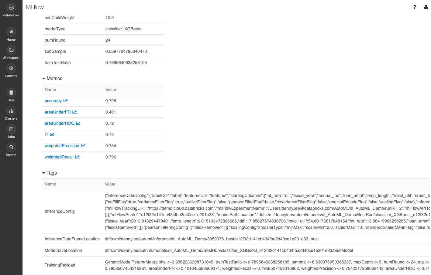
As noted in the MLflow details (preceding screenshot), the AUC (areaUnderROC) has improved to a value of 0.72!
How did the AutoML Toolkit do this? The details behind how the AutoML Toolkit was able to do this will be discussed in a future blog. From a high level, the AutoML toolkit was able to find much better hyperparameters because it tested and tuned all modifiable hyperparameters in a distributed fashion using a collection of optimization algorithms. Incorporated within AutoML toolkit is the understanding of how to use the parameters extracted from the algorithm source code (e.g. XGBoost in this case).
Clearing up the Confusion
With the remarkable improvement in the AUC value, how much better does the AutoML XGBoost model perform in comparison to the hand created one? Because this is a binary classification problem, we can clear up the confusion using confusion matrices. The confusion matrices from both the hand-made model and AutoML Toolkit notebooks are included below. To match the analysis of what we did in the past (ala Loan Risk Analysis with XGBoost and Databricks Runtime for Machine Learning), we’re evaluating for loans that were issued after 2015.
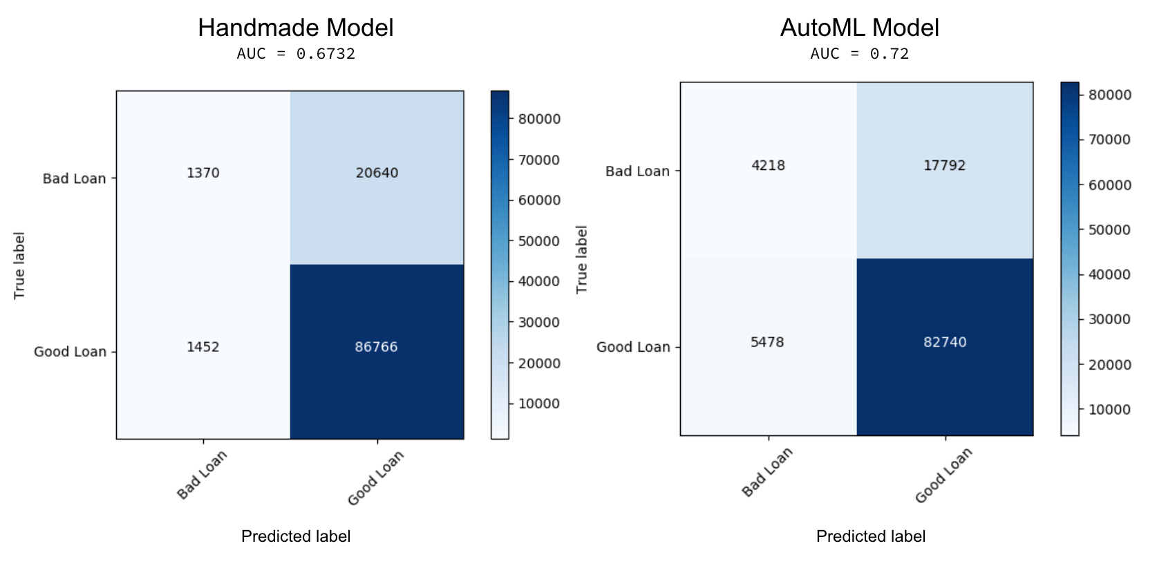
In the preceding graphic, the confusion matrix on the left is from the hand-made XGBoost model while the one on the right is from AutoML Toolkit. While both models do a great job correctly identifying good loans (True: Good, Predicted: Good), the AutoML model performs better on identifying bad loans (True: Bad, Predicted: Bad – 4218 vs. 1370) as well as preventing false positives (True: Bad, Predict: Good – 17792 vs. 20640). In this scenario, this would mean that if we were to have used the machine learning model created by AutoML (as opposed to the handmade model), we could have potentially prevented issuing 2848 more bad loans that would have likely defaulted and cost money. Just as important, this model potentially would have prevented even more headaches and a bad customer experience by lowering the false positives - incorrectly predicting this was a good loan when in fact it was likely a bad loan.
Understanding the Business Value
Let’s quantify this confusion matrix to business value; the definition would be:
| Prediction | Label (Is Bad Loan) | Short Description | Long Description |
|---|---|---|---|
| 1 | 1 | Loss Avoided | Correctly found bad loans |
| 1 | 0 | Profit Forfeited | Incorrectly labeled bad loans |
| 0 | 1 | Loss Still Incurred | Incorrectly labeled good loans |
| 0 | 0 | Profit Retained | Correctly found good loans |
To review the dollar value associated with our confusion matrix for our hand-made model, we will use the following code snippet.
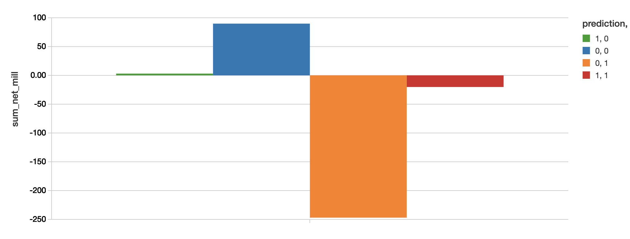
To review the dollar value associated with our confusion matrix of the AutoML Toolkit model will use the following code snippet.
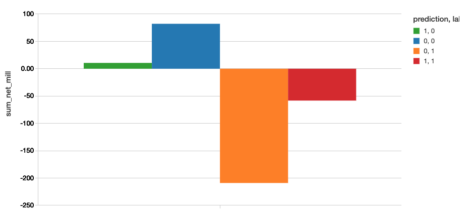
Business value is calculated as value = -(loss avoided - profit forfeited)
| Model | Loss Avoided | Profit Forfeited | Value |
|---|---|---|---|
| Hand Made | -20.16 | 3.06 | $23.22M |
| AutoML Toolkit | -58.22 | 10.66 | $68.88M |
As you can observe, the potential profits saved by using the AutoML Toolkit is 3x better than our handmade model with savings of $68.88M.
AutoML Toolkit: Less Code and Faster
With the AutoML Toolkit, you can write less code to deliver better results faster. For this loan risk analysis with XGBoost example, we had seen an improvement in performance of AUC = 0.72 vs. 0.6732 (potential savings of $68.88M vs. $23.22M with the original technique). The AutoML toolkit was able to find much better hyperparameters because it automatically generated, tested, and tuned all of the algorithm’s modifiable hyperparameters in a distributed fashion.
Try out the AutoML Toolkit with the Using AutoML Toolkit to Simplify Loan Risk Analysis XGBoost Model Optimization notebook on Databricks today!
Corrections
Previously this blog has stated an AUC value of 0.995 due to mistakenly keeping the net column for feature generation (it has an almost 1:1 relationship with loan prediction). Once this was corrected, the correct AUC is 0.72. Thanks to Sean Owen, Sanne De Roever, and Carsten Thone who quickly identified this issue.
Get the latest posts in your inbox
Subscribe to our blog and get the latest posts delivered to your inbox.