Optimizing User Defined Functions with Apache Spark™ and R in the Real World: Scaling Pitch Scenario Analysis with the Minnesota Twins Part 2

Introduction

In part 1 we talked about how Baseball Operations for the Minnesota Twins wanted to run up to 20k simulations on 15 million historical pitches - 300 billion total simulations -  to more accurately evaluate player performance.  The idea is simple:  if 15 million historical pitches sketched an image of player performance, 300 billion simulated pitches from each players’ distribution would sharpen that image and provide more reliable valuations.  This data would impact coaching and personnel decisions with the goal of generating more wins, and by extension, revenue for the club.

All of the scripts and machine learning models to generate and score data were written in R.  Even when running these scripts with multi-threading packages in R they estimated it would take 3.8 years to process all of the simulations.  With user defined functions (UDFs) in Apache Spark and Databricks we were able to reduce the data processing time to 2-3 days for 300 billion simulations on historical data sets, and near real time for in-game data. By enabling near real-time scoring of in-game pitches, the Twins are looking to eventually optimize lineup and strategy decisions based on in-game conditions, for example, choosing the best pitcher and pitch given the batter, weather, inning, and speed + rotation readings from the pitcher’s last throws.

By combining the vast ecosystem of R packages with the scalability and parallelism of Spark, UDFs can be extraordinarily powerful not just in sports but across industry use cases.  In addition to our model inference use case for the Twins, consider the following applications:

• Generating sales forecasts for thousands of consumer products using time series packages like prophet
• Simulating the performance of hundreds of financial portfolios
• Simulating transportation schedules for fleets of vehicles
• Finding the best model fit by searching thousands of hyperparameters in parallel

As exciting and tantalizing as these applications are, their power comes at a cost.  Ask anyone who has tried and they will tell you that implementing a UDF that can scale gracefully can be quite challenging.   This is due to the need to efficiently manage cores and memory on the cluster, and the tension between them.  The key is to structure the job in such a way that Spark can linearly scale it.

In this post we embark on a journey into what it takes to craft UDFs that scale.  Success hinges on an understanding of storage, Spark, R, and the interactions between them.

Understanding UDFs with Spark and R

Generally speaking, when you use SparkR or sparklyr your R code is translated into Scala, Spark’s native language.  In these cases the R process is limited to the driver node of the Spark cluster, while the rest of the cluster completes tasks in Scala.  User defined functions, however, provide access to an R process on each worker, letting you apply an R function to each group or partition of a Spark DataFrame in parallel before returning the results.

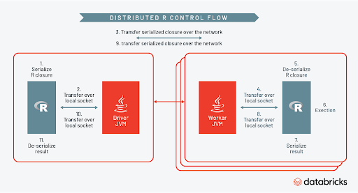
How does Spark orchestrate all of this?  You can see the control flow clearly in the diagram below.

As part of each task Spark will create a temporary R session on each worker, serialize the R closure, then distribute the UDF across the cluster.  While the R session on each worker is active, the full power of the R ecosystem can be leveraged inside the UDF.  When the R code is finished executing the session is terminated, and results sent back to the Spark context.  You can learn more about this by watching the talk here and in this blog post.

Getting UDFs Right

“...you will be fastest if you avoid doing the work in the first place.” [1] 

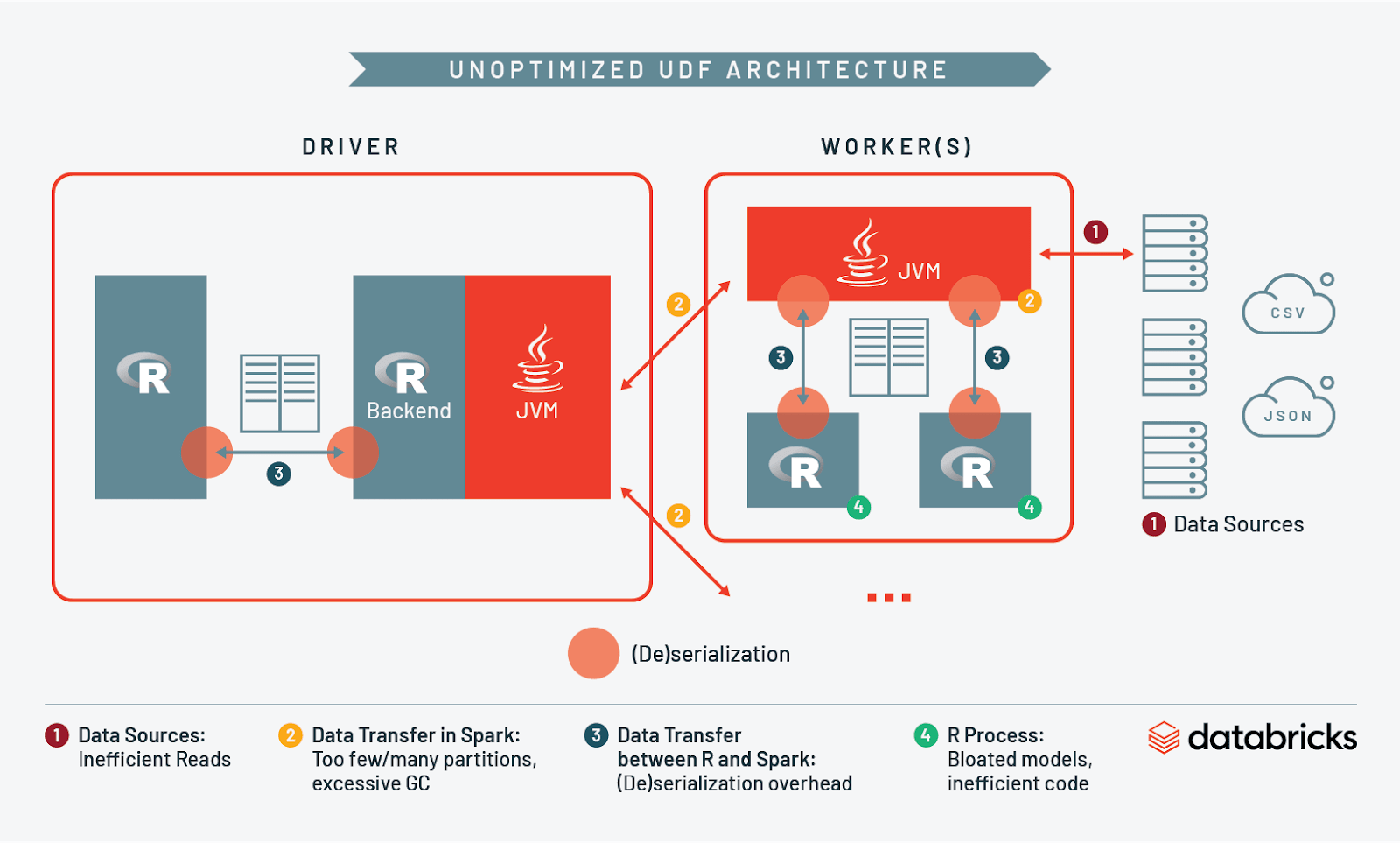
Now that we understand the basics of how UDFs are executed, let’s take a closer look at potential bottlenecks in the system and how to eliminate them.  There are essentially four key areas to understand when writing these functions:

1. Data Sources
2. Data Transfer in Spark
3. Data Transfer Between Spark and R
4. R Process

1. Data Sources: Minimizing Storage I/O

The first step is to plan how data is organized in storage.  Many R users may be used to working with flat files, but a key principle is to only ingest what is necessary for the UDF to execute properly. A significant portion of your job will be I/O to and from storage, and if your data is currently in an unoptimized file format (like CSV) Spark may need to read the entire data set into memory.  This can be painfully slow and inefficient, particularly if you don’t need all of the contents of that file.

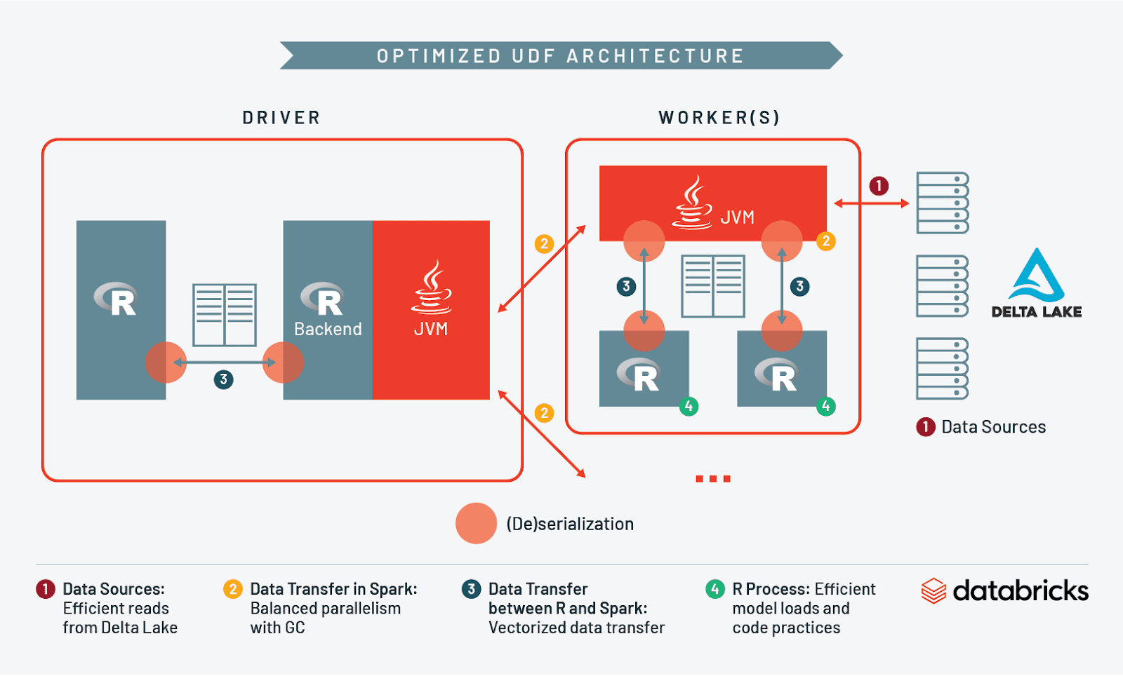
For this reason we recommend saving your data in a scalable format like Delta Lake.  Delta speeds up ingestion into Spark by partitioning data in storage, optimizing the size of these partitions, and creating a secondary index with Z-Ordering.  Taken together, these features help limit the volume of data that needs to be accessed in a UDF.

How so?  Imagine we partitioned our baseball data in storage by pitch type and directed Spark to read rows where pitch type equals ‘curveball’.  Using Delta we could skip the ingestion of all rows with other pitch types.  This reduction in the scan of data can speed up reads tremendously - if only 10% of your data contains curveball pitches, you can effectively skip reading 90% of your dataset into memory!

By using a storage layer like Delta Lake and a partitioning strategy that corresponds to what data will be processed by the UDF, you will have laid a solid foundation and eliminated a potential bottleneck to your job.

2a. Data Transfer in Spark: Optimizing Partition Size in Memory

The size of partitions in memory can affect performance of feature engineering/ETL pipelines leading up to and including the UDF itself.   In general, whenever Spark has to perform a wide transformation like a join or group by, data must be shuffled across the cluster.The default setting for the number of shuffle partitions is arbitrarily set to 200, meaning at the time of a shuffle operation the data in your Spark DataFrame is distributed across 200 partitions.

This can create inefficiencies depending on the size of your data.  If your dataset is smaller, 200 partitions may be over-parallelizing the work, causing unnecessary scheduling overhead and tasks with very little data in them.  If the dataset is large you may be under-parallelizing and not effectively using the resources on your cluster.

As a general rule of thumb, keeping the size of shuffle partitions between 128-200MB will maximize parallelism while avoiding spilling data to disk.  To identify how many shuffle partitions there should be, use the Spark UI for your longest job to sort the shuffle read sizes.  Divide the size of the largest shuffle read stage by 128MB to arrive at the optimal number of partitions for your job.  Then you can set the spark.sql.shuffle.partitions config in SparkR like this:

Actively repartitioning a Spark DataFrame is also impacted by this setting as it requires a shuffle.  As we’ll see, this behavior can be used to manage memory pressure in other parts of the system like garbage collection and data transfer between Spark and R.

2b. Data Transfer in Spark: Garbage Collection and Cluster Sizing

When you have a big data problem it can be tempting to adopt a brute force approach and reach for the largest worker type, but the solution may not be so simple.  Garbage collection in the Java Virtual Machine (JVM) tends to get out of control when there are large objects in memory that are no longer being used.  Using very large workers can exacerbate this problem because there’s more room to create large objects in the first place.  Managing the size of objects in memory is thus a key consideration of the solution architecture.

For this particular job we found that a few large workers or many small workers did not perform as well as many medium sized workers.  Large workers would generate excessive garbage collection causing the job to hang indefinitely, while small workers would simply run out of memory.

To address this we gradually increased the size of workers until we wound up in the middle range of RAM and CPU that JVM garbage collection can gracefully handle.  We also repartitioned the input Spark DataFrame to our UDF and increased its partitions.  Both measures were effective at managing the size of objects in the JVM and helped keep garbage collection to less than 10% of the total task time for each Spark executor.  If we wanted to score more records we could simply add more medium-sized workers to the cluster and increase the partitions of the input DataFrame in a linear fashion.

3. Data Transfer between Spark and R

The next step to consider was how data is passed between Spark and R.Here we identified two potential bottlenecks - overall I/O and the corresponding (de)serialization that occurs between processes.

First, only input what is necessary for the UDF to execute properly.  Similar to how we optimize I/O reads from storage, filter the input Spark DataFrame to contain only those columns necessary for the UDF. If our Spark DataFrame has 30 columns and we only need 4 of them for the UDF, subset your data accordingly and use that as input instead.  This will speed up execution by reducing I/O and related (de)serialization.

If you’ve subset the input data appropriately and still have out-of-memory issues, repartitioning can help control how much data is transferred between Spark and R.  For example, applying a UDF to 200GB of data across 100 partitions will result in 2GB of data sent to R in each task.  If we increase the number of partitions to 200 using the `repartition()` function from SparkR, then 1 GB will be sent to R in each task.  The tradeoff of more partitions is more (de)serialization tasks between the JVM and R, but less data and subsequent memory pressure in each task.

You might think a typical 14GB RAM Spark worker would be able to handle a 2GB partition of data with room to spare, but in practice you will require at least 30GB RAM if you want to avoid out-of-memory errors!  This can be a rude awakening for many developers trying to get started with UDFs in Spark and R, and can cause costs to skyrocket.  Why do the workers need so much memory?

The fact is that Spark and R represent data in memory quite differently.  To transfer data from Spark to R, a copy must be created and then converted to an in-memory format that R can use.  Recall that in the UDF architecture diagram above, objects need to be serialized and deserialized every time they move between the two contexts.  This is slow and creates enormous memory overhead, with workers typically requiring an order of magnitude greater memory than expected.

We can mitigate this bottleneck by replacing the two distinct in-memory formats with a single one using Apache Arrow.   Arrow is designed to quickly and efficiently transfer data between different systems - like Spark and R - by using a columnar format similar to Parquet.  This eliminates the time spent in serialization/deserialization as well as the increased memory overhead.  It is not uncommon to see speed-ups of 10-100x when comparing workloads with vs. without Arrow.  It goes without saying that using one of these optimizations is critical when working with UDFs.  Spark 3.0 will include support for Arrow in SparkR, and you can install Arrow for R on Databricks by following the instructions here.  It’s also worth noting that there is a similar out-of-the-box optimizer  available for SparkR on Databricks Runtime.

4. R Process: Managing Idiosyncrasies of R

Each language has its own quirks, and so now we turn our attention to R itself.  Consider that the function in your UDF may be applied hundreds or thousands of times on the workers, so it pays to be mindful of how R is using resources.

In tuning the pitch scoring function we identified loading the model object and commands that trigger R’s copy-on-modify behavior as potential bottlenecks in the job.  How’s that?  Let’s examine these two more carefully, beginning with loading the model object.

If you’ve worked with R long enough, you probably know that many R packages include training data as part of the model object.  This is fine when the data is small, but when the data grows it can become a significant problem - some of the pitch models were nearly 2GB in size!   In our case the overhead associated with loading and dropping these models from memory in each execution of the UDF limited the scale to 300 million rows, 3 orders of magnitude away from 300 billion.

Furthermore, we noticed that the model had been saved as part of a broader training function:

By efficiently loading model objects into memory and eliminating copy-on-modify behavior we streamlined R’s execution within the UDF.

Testing, Debugging and Monitoring

Understanding how to begin testing, debugging and monitoring your UDF is just as important as knowing how the system works.  Here are some tips to get started.

For testing, it is best to start by simply counting rows in each group or partition of data, making sure every row is flowing through the UDF.  Then take a subset of input data and start to slowly introduce additional logic and the results that you return until you get a working prototype.  Finally, slowly scale up the execution by adding more rows until you’ve submitted all of them.

At some point you will almost certainly hit errors and need to debug. If the error is with Spark you will see the stack trace in the console of the driver.  If the error is with your R code inside the UDF, this will not be shown in the driver output.  You’ll need to open up the Spark UI and check stderr from the worker logs to see the stack trace from the R process.

Once you have an error free UDF, you can monitor the execution using Ganglia metrics.  Ganglia contains detailed information on how and where the cluster is being utilized and can provide valuable clues to where a bottleneck may lie.  For the pitch scoring pipeline, we used Ganglia to help diagnose multiple issues - we saw CPU idle time explode when model objects were too large, and eliminated swap memory utilization when we increased worker size.

Putting it All Together

At this point we have discussed I/O and resource management when reading into Spark, across workers, between Spark and R, and in R itself.  Let’s take what we’ve learned and compare what an unoptimized architecture looks like vs. an optimized one:

Conclusion

At the beginning of this post, we stated that the key to crafting a UDF with Spark and R is to structure the job in such a way that Spark can linearly scale it. In this post we learned about how to scale a model scoring UDF by optimizing each major component of the architecture - from storing data in Delta Lake, to data transfer in Spark, to data transfer between R and Spark, and finally to the R process itself.  While all UDFs are somewhat different, R developers should now feel confident in their ability to navigate this pattern and avoid major stumbling blocks along the way.