Model Evaluation in MLflow

Many data scientists and ML engineers today use MLflow to manage their models. MLflow is an open-source platform that enables users to govern all aspects of the ML lifecycle, including but not limited to experimentation, reproducibility, deployment, and model registry. A critical step during the development of ML models is the evaluation of their performance on novel datasets.

Motivation

Why Do We Evaluate Models?

Model evaluation is an integral part of the ML lifecycle. It enables data scientists to measure, interpret, and explain the performance of their models. It accelerates the model development timeframe by providing insights into how and why models are performing the way that they are performing. Especially as the complexity of ML models increases, being able to swiftly observe and understand the performance of ML models is essential in a successful ML development journey.

State of Model Evaluation in MLflow

Currently, many users evaluate the performance of their MLflow model of the python_function (pyfunc) model flavor through the mlflow.evaluate API, which supports the evaluation of classification and regression models. It computes and logs a set of built-in task-specific performance metrics, model performance plots, and model explanations to the MLflow Tracking server.

To evaluate MLflow models against custom metrics not included in the built-in evaluation metric set, users would have to define a custom model evaluator plugin. This would involve creating a custom evaluator class that implements the ModelEvaluator interface, then registering an evaluator entry point as part of an MLflow plugin. This rigidity and complexity could be prohibitive for users.

According to an internal customer survey, 75% of respondents say they frequently or always use specialized, business-focused metrics in addition to basic ones like accuracy and loss. Data scientists often utilize these custom metrics as they are more descriptive of business objectives (e.g. conversion rate), and contain additional heuristics not captured by the model prediction itself.

In this blog, we introduce an easy and convenient way of evaluating MLflow models on user-defined custom metrics. With this functionality, a data scientist can easily incorporate this logic at the model evaluation stage and quickly determine the best-performing model without further downstream analysis.

*Note: In MLflow 2.4, mlflow.evaluate is expanded to support LLM text, text summarization, and question answering models

Usage

Built-in Metrics

MLflow bakes in a set of commonly used performance and model explainability metrics for both classifier and regressor models. Evaluating models on these metrics is straightforward. All we need is to create an evaluation dataset containing the test data and targets and make a call to mlflow.evaluate.

Depending on the type of model, different metrics are computed. Refer to the Default Evaluator behavior section under the API documentation of mlflow.evaluate for the most up-to-date information regarding built-in metrics.

Example

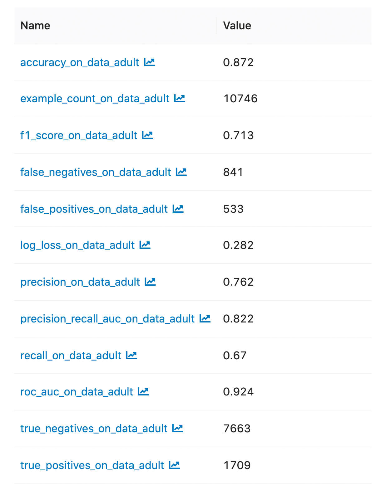
Below is a simple example of how a classifier MLflow model is evaluated with built-in metrics.

First, import the necessary libraries

Then, we split the dataset, fit the model, and create our evaluation dataset

Finally, we start an MLflow run and call mlflow.evaluate

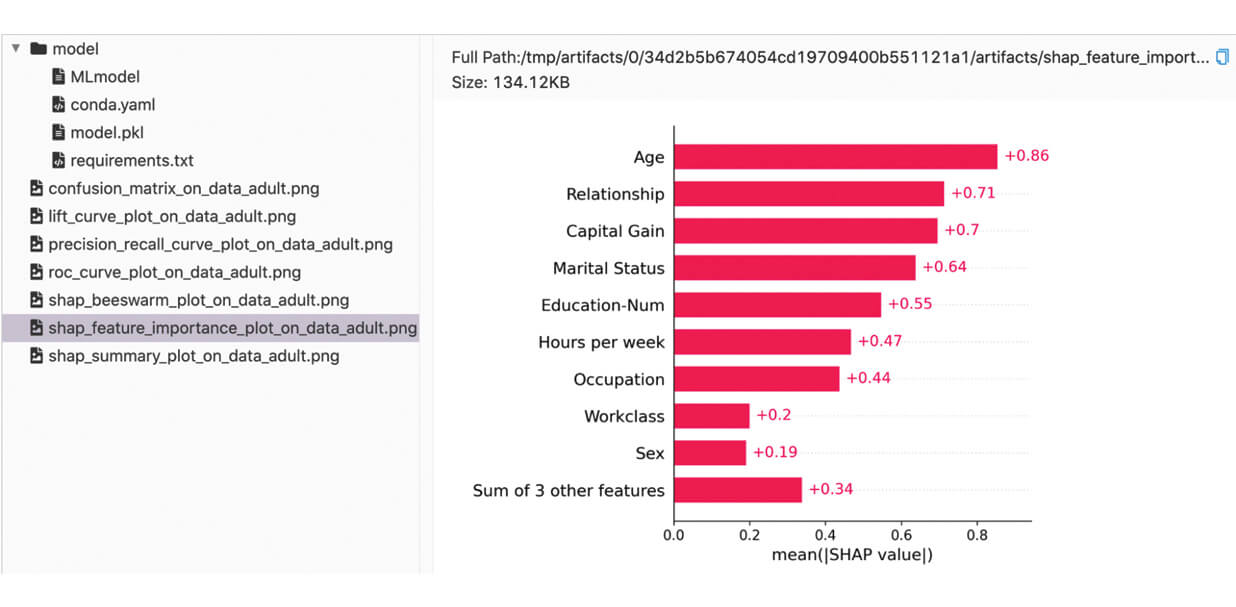
We can find the logged metrics and artifacts in the MLflow UI:

Custom Metrics

To evaluate a model against custom metrics, we simply pass a list of custom metric functions to the mlflow.evaluate API.

Function Definition Requirements

Custom metric functions should accept two required parameters and one optional parameter in the following order:

1. eval_df: a Pandas or Spark DataFrame containing a prediction and a target column.

   E.g. If the output of the model is a vector of three numbers, then the eval_df DataFrame would look something like: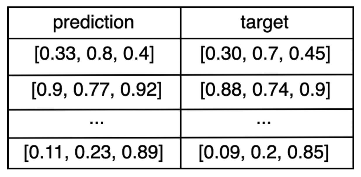

   

2. builtin_metrics: a dictionary containing the built-in metrics

   E.g. For a regressor model, builtin_metrics would look something like:
3. (Optional) artifacts_dir: path to a temporary directory that can be used by the custom metric function to temporarily store produced artifacts before logging to MLflow.

   E.g. Note that this will look different depending on the specific environment setup. For example, on MacOS it look something like this:

   If file artifacts are stored elsewhere than artifacts_dir, ensure that they persist until after the complete execution of mlflow.evaluate.

Return Value Requirements

The function should return a dictionary representing the produced metrics and can optionally return a second dictionary representing the produced artifacts. For both dictionaries, the key for each entry represents the name of the corresponding metric or artifact.

While each metric must be a scalar, there are various ways to define artifacts:

• The path to an artifact file
• The string representation of a JSON object
• A pandas DataFrame
• A numpy array
• A matplotlib figure
• Other objects will be attempted to be pickled with the default protocol

Refer to the documentation of mlflow.evaluate for more in-depth definition details.

Example

Let’s walk through a concrete example that uses custom metrics. For this, we’ll create a toy model from the California Housing dataset.

Then, setup our dataset and model

Here comes the exciting part: defining our custom metrics function, and a custom artifact!!

Finally, to tie all of these together, we’ll start an MLflow run and call mlflow.evaluate:

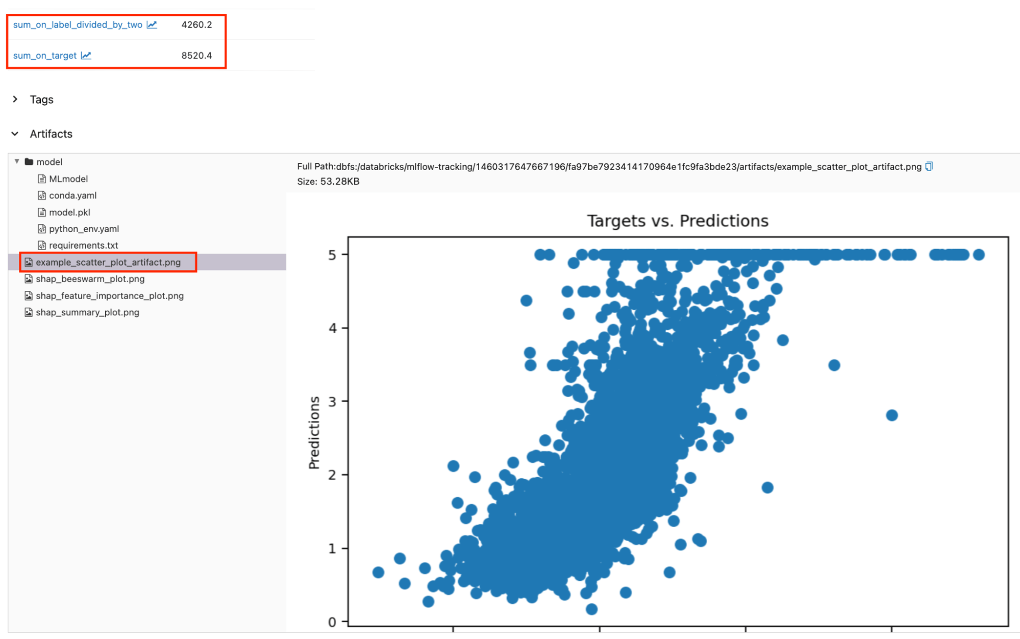
Logged custom metrics and artifacts can be found alongside the default metrics and artifacts. The red boxed regions show the logged custom metrics and artifacts on the run page.

Accessing Evaluation Results Programmatically

So far, we have explored evaluation results for both built-in and custom metrics in the MLflow UI. However, we can also access them programmatically through the EvaluationResult object returned by mlflow.evaluate. Let’s continue our custom metrics example above and see how we can access its evaluation results programmatically. (Assuming result is our EvaluationResult instance from here on).

We can access the set of computed metrics through the result.metrics dictionary containing both the name and scalar values of the metrics. The content of result.metrics should look something like this:

Similarly, the set of artifacts is accessible through the result.artifacts dictionary. The values of each entry is an EvaluationArtifact object. result.artifacts should look something like this:

Example Notebooks

• Short Example
• Comprehensive Example

Underneath the Hood

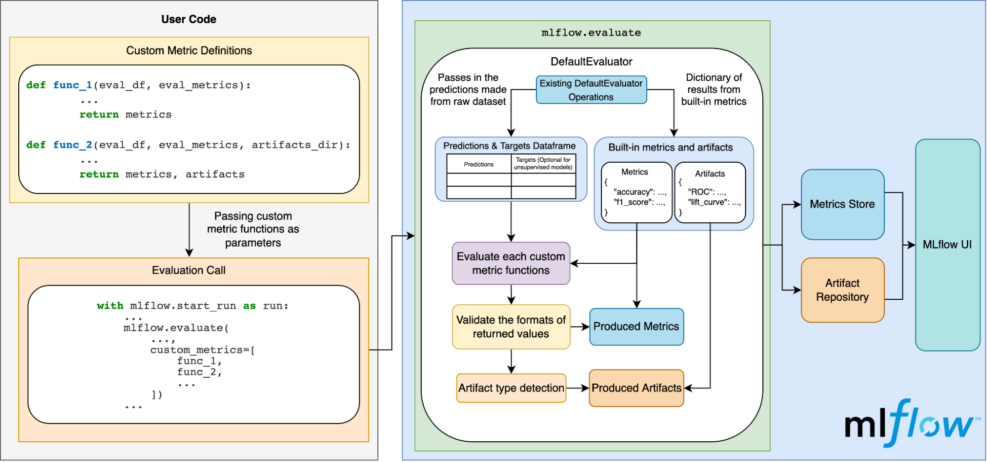
The diagram below illustrates how this all works under the hood:

Conclusion

In this blog post, we covered:

• The significance of model evaluation and what’s currently supported in MLflow.
• Why having an easy way for MLflow users to incorporate custom metrics into their MLflow models is important.
• How to evaluate models with default metrics.
• How to evaluate models with custom metrics.
• How MLflow handles model evaluation behind the scenes.