
How long should you train your language model? How large should your model be? In today's generative AI landscape, these are multi-million dollar questions.
Over the last few years, researchers have developed scaling laws, or empirical formulas for estimating the most efficient way to scale up the pretraining of language models. However, popular scaling laws only factor in training costs, and ignore the often incredibly expensive costs of deploying these models. Our recent paper, presented at ICML 2024, proposes a modified scaling law to account for the cost of both training and inference. This blog post explains the reasoning behind our new scaling law, and then experimentally demonstrates how “overtrained” LLMs can be optimal.
The “Chinchilla” Scaling Law is the most widely cited scaling law for LLMs. The Chinchilla paper asked the question: If you have a fixed training compute budget, how should you balance model size and training duration to produce the highest quality model? Training costs are determined by model size (parameter count) multiplied by data size (number of tokens). Larger models are more capable than smaller ones, but training on more data also improves model quality. With a fixed compute budget, there is a tradeoff between increasing model size vs. increasing training duration. The Chinchilla authors trained hundreds of models and reported an optimal token-to-parameter ratio (TPR) of roughly 20. This “Chinchilla optimal” value of ~20 tokens/parameter quickly became the industry standard (for example, later models such as Cerebras-GPT and Llama-1 65B were trained using Chinchilla scaling).
Once the model has completed training, it needs to be deployed. Since LLM serving costs are a function of the model size (in addition to user demand), larger models are much more expensive to deploy. Model size is therefore an important cost factor for both training and inference time.
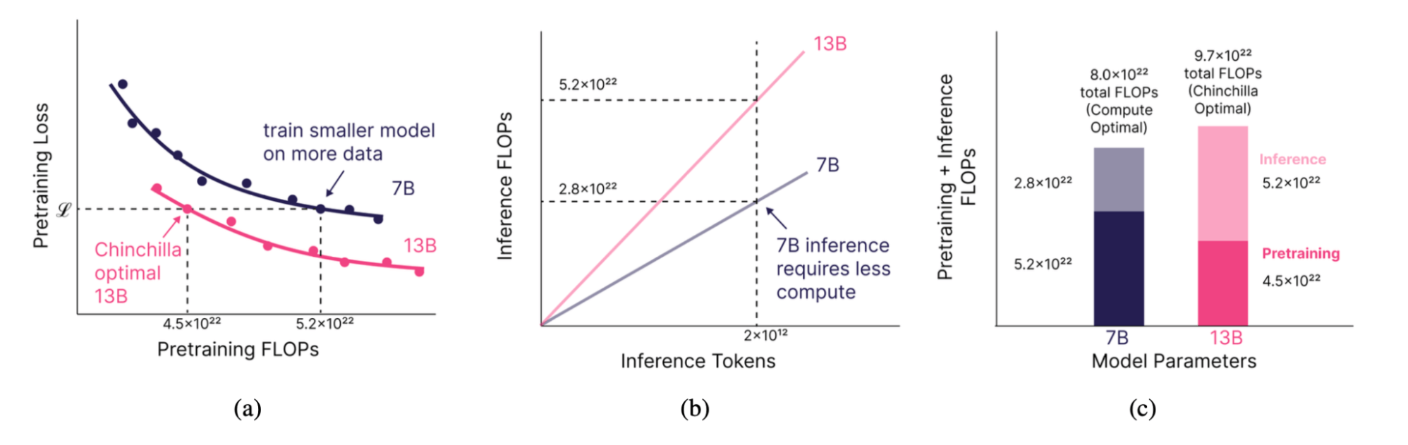
In our research, we were motivated by the idea of training smaller models on more data than the Chinchilla law suggested. By spending extra money on training to produce a smaller but equivalently powerful model, we predicted that we could make up for these extra training costs at inference time (Fig. 1). How much smaller? That depends on just how much inference demand we anticipate.
Our adjusted scaling law returns the most efficient way to train and deploy a model based on desired quality and expected inference demand. Our scaling law quantifies the training-inference trade-off, producing models that are optimal over their total lifetime.
The more inference demand you expect from your users, the smaller and longer you should train your models. But can you really match the quality of a large model with a smaller one trained on far more data? Some have postulated that there is a critical model size below which it is not possible to train on any number of tokens and match a Chinchilla-style model.
To answer this question and validate our method, we trained a series of 47 models of different sizes and training data lengths. We found that model quality continues to improve as we increase tokens per parameter to extreme ranges (up to 10,000 tokens/parameter, or 100x longer than typical), although further testing is needed at extreme scales.
Since we first published a version of this work in December 2023, it has become more common to train models for much longer durations than the Chinchilla optimal ratio. This is exemplified by successive generations of LLaba models: while the Llama-1 65B model released in February 2023 was trained with ~20 tokens/parameter (1.4 trillion tokens), Llama-2-70B was trained for almost 30 tokens/parameter (2 trillion), and Llama-3-70B was trained for over 200 tokens/parameter (15 trillion)! This trend is driven in part by the wild popularity of powerful, smaller models in the 1B - 70B parameter range that are easier and cheaper to finetune and deploy.
The Details: How Scaling Laws Can Account for Both Training and Inference
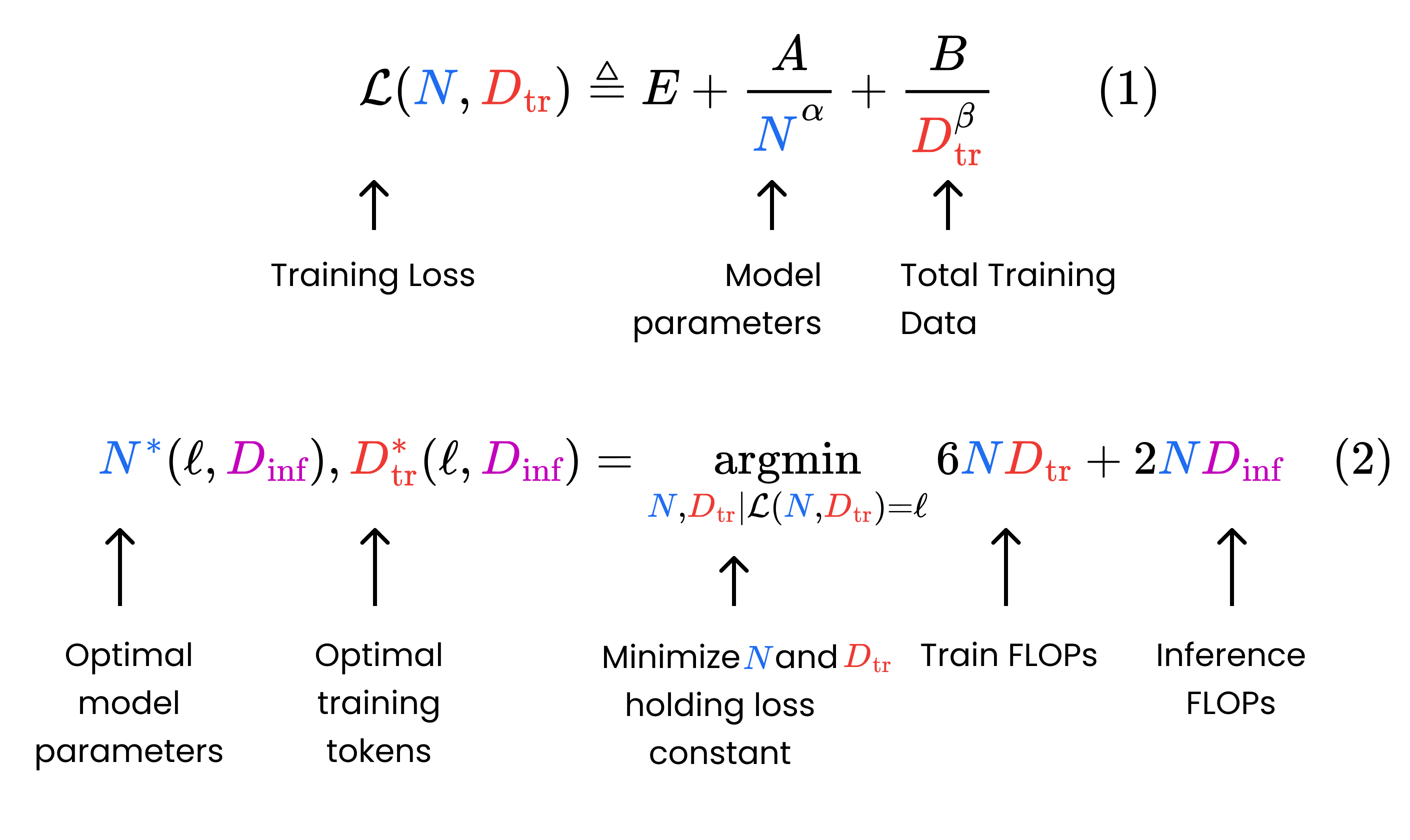
The Chinchilla paper presented a parametric function (Fig. 2, Eq. 1) for model loss in terms of the number of model parameters and training tokens. The authors trained a large set of models to empirically find the best-fit values for the coefficients in Equation 1. Then, they developed a formula to minimize this function (lower loss = higher quality model) subject to a fixed training compute budget, where compute is measured in terms of floating-point operations (FLOPs).
By contrast, we assume a fixed pretraining loss (i.e. model quality) and find the model size and training duration that minimize the total compute over the model’s lifetime, including both training and inference (Fig. 2, Eq. 2).
We believe our setup is more closely aligned with how teams think about developing LLMs for production. In practice, organizations care deeply about ensuring their model reaches a certain quality. Only if it hits their evaluation metrics can they then deploy it to end users. Scaling laws are useful inasmuch as they help minimize the total cost required to train and serve models that meet those metrics.
For example, suppose you’re looking to train and serve a 13B Chinchilla-quality model, and you anticipate 2 trillion tokens of inference demand over the model’s lifetime. In this scenario, you should instead train a 7B model on 2.1x the training data until it reaches 13B quality, and serve this 7B model instead. This will reduce the compute required over your model’s lifetime (training + inference) by 17% (Figure 1).
How Long Can You Really Train?
In high-demand inference scenarios, our scaling law suggests that we should train significantly smaller models on much more data than Chinchilla indicates, producing data/model ratios of hundreds or even thousands of tokens per parameter. However, scaling laws haven’t been validated at these outer ranges. Most researchers conduct experiments only at typical (<~100 tokens/parameter) ratios. Can models really keep learning if you train them for that long?
To characterize transformer behavior at extreme data sizes, we trained 47 LLMs with the MPT architecture, with varying size and token ratios. Our models ranged from 150M to 6B parameters, and our data budgets ranged from 10 to 10,000 tokens per parameter. Due to resource constraints, we could not complete a full sweep for all model sizes (e.g. we trained our 2.5B model on up to 500 tokens/parameter).
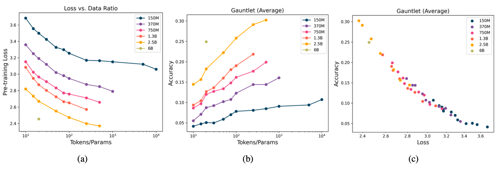
Our key experimental finding is that loss continues to decrease (i.e. model quality improves) as we increase tokens per parameter, even to extreme ratios. Although it takes exponentially more tokens to reduce loss at large ratios, loss does not plateau as we scale to 10,000 tokens per parameter for our 150M model. We find no evidence of a “saturation point” for LLMs, although further testing is needed at extreme scales.
In addition to model loss, we also considered downstream metrics. We evaluated each model on a version of our open source Mosaic Evaluation Gauntlet, which consists of 50-odd tasks in five different categories: World Knowledge (e.g. MMLU), Commonsense Reasoning (e.g. BIG-bench), reading comprehension (SQuAD), language understanding (e.g. LAMBADA), and symbolic problem solving (e.g. GSM-8k). Our downstream metrics also improved as we trained longer and longer.
Loss and Gauntlet Average are tightly correlated (Fig 3(c)), showing that improvements in loss are excellent predictors of improvements in general model quality. LLM developers interested in predicting downstream metrics as a function of model parameters and token counts can use loss as a proxy for their aggregate results and take advantage of existing scaling laws to accurately understand how their downstream metrics change at scale.
Estimating Real-World Costs of Training and Inference
Thus far, our proposed scaling law purely optimizes for minimum total (training + inference) FLOPs. However, in practice, we care far more about minimizing costs rather than compute, and the cost of a training FLOP is different from the cost of an inference FLOP. Inference is run on different hardware, with different prices, and at different utilizations.
To make our method more applicable to real-world deployments, we modified our objective in Fig. 2. Instead of minimizing FLOPs, we minimized cost. To produce a good cost estimate, we split off training, prefill (processing prompts), and decoding (output generation) and estimated costs for each stage. Although our method simplifies how things work in the real world, it’s flexible enough to account for different hardware types and utilization.
Adjusting our method from compute-optimal to cost-optimal can profoundly impact our recommendations. For example, assuming realistic numbers for training, prompt processing, and output generation, a Chinchilla-style 70B model is only 1% off the compute-optimal model for the same inference demand of 2 trillion tokens, but costs 36% more than a cost-optimal model.
Conclusion
Our research modifies scaling laws to account for the computational and real-world costs of both training and inference. As inference demand grows, the additional cost pushes the optimal training setup toward smaller and longer-trained models.
We experimentally validated the hypothesis that very small models, trained on enough data, can match larger ones trained to their Chinchilla ratio (20x tokens/parameter). Our results show that LLM practitioners operating in inference-heavy regimes can (and often should!) train models considerably longer than the current literature suggests and continue to see quality improvements.
Finally, this work inspired our development of DBRX, a Databricks Mixture-of-Experts model with 132B total parameters trained for 12 trillion tokens. Want to train your own models? Contact us! At Databricks Mosaic AI, we conduct LLM research like this so you can train high-quality, performant models more efficiently on our platform.
Interested in developing language models and sharing insights about them? Join Databricks Mosaic AI! We have open engineering and research positions.
Notes and Further Reading
This research was first published in early form in December 2023 at the NeurIPS 2023 Workshop on Efficient Natural Language and Speech Processing. It will be presented in July 2024 at the International Conference on Machine Learning. The full research paper may be viewed at this link: Beyond Chinchilla-Optimal: Accounting for Inference in Language Model Scaling Laws.
Many studies have contributed to the development of scaling laws for LLMs, including Hestness et al. (2017; 2019), Rosenfeld et al. (2019), Henighan et al. (2020), Kaplan et al. (2020), Sorscher et al. (2022), and Caballero et al. (2022) (see Villalobos (2023) for a review). Some of these studies focused on scaling laws for transfer settings (i.e. downstream performance), such as Hernandez et al. (2021); Mikami et al. (2021); Abnar et al. (2021) and Tay et al. (2022).
A few studies such as Besiroglu et al. (2024) and Porian et al. (2024) have also further scrutinized the parametric function fitting approach of the original Chinchilla paper by Hoffman et al. 2022.
A handful of exciting scaling law papers have been published since 2023, when an earlier version of this work was presented (Sardana and Frankle 2023). For example, Krajewski et al. (2024) characterize differences in scaling properties between dense transformers and Mixture of Expert (MoE) models. More theoretical studies include Michaud et al. (2024), Bordelon et al. (2024), Paquette et al. (2024) and Ruan et al. (2024).
The results presented in Gadre et al. (2024) are particularly relevant to this paper. The authors train 100 models between the sizes of 1.4B and 6.9B parameters and on data with tokens-per-parameter ratios between 20 and 640. Similar to our study, they find reliable scaling laws in these model and data regimes. They also find that downstream task performance is strongly correlated to LLM perplexity.