Implementing a dimensional data warehouse with Databricks SQL: Part 1
Defining the data objects

Summary
- Implement dimensional data warehouses in Databricks SQL to optimize for fast query performance.
- The physical model structure in Databricks SQL, including creating dimension and fact tables, is done with SQL CREATE TABLE statements.
- It is important to add descriptive comments to tables and columns for better metadata management.
More and more organizations are moving their data warehouse workloads to Databricks. The platform's elastic nature and significant enhancements to its query execution engine have allowed Databricks to set world records for both data warehouse query performance and cost performance, making it an increasingly appealing option for analytics infrastructure consolidation.
To support these efforts, we’ve previously blogged about how Databricks support various data warehouse design approaches. In this blog series, we want to take a closer look at one of the most popular approaches to data warehousing, dimensional modeling, a design pattern characterized by star- and snowflake schemas, and dive deep into the standardized extraction, transformation and loading (ETL) patterns widely adopted in support of this approach.
To make this widely accessible to the dimensional modeling community, we will adhere closely to the classic patterns associated with this modeling approach. This information will be spread across the following blog posts:
- Part 1: Defining the (Dimensional) Data Objects (this post)
- Part 2: Building the Dimension ETL Workflows
- Part 3: Building the Fact ETL Workflows
In addition, we will center our design discussions around one of the more commonly used star schemas (Figure 1) in the AdventureWorksDW database, a sample database created by Microsoft and widely used for data warehouse and Business Intelligence training purposes.
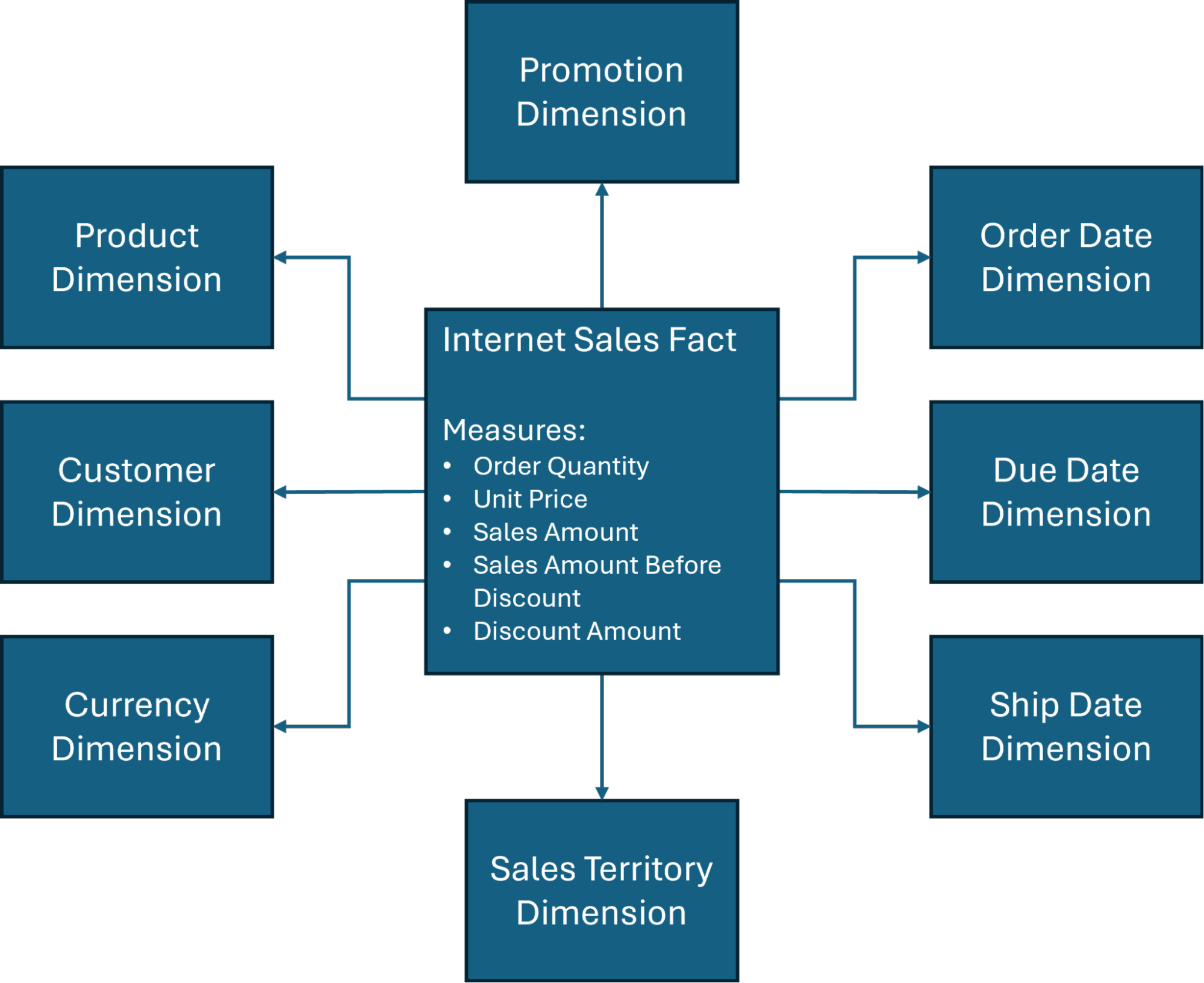
What is dimensional modeling in data warehousing?
Dimensional modeling optimizes data storage for fast query performance. By structuring data into facts and dimensions, you can easily analyze data from multiple perspectives. It also enables you to explore data from various angles simultaneously (multidimensional analysis).
What are the four dimensions of a data warehouse?
As Figure 1 indicates, there are several dimensions involved in the star schema of data warehousing, but the four primary dimensions of data warehousing typically include the following:
Time: This provides a historical tracking framework and it’s essential for evaluating trends or conducting comparisons. You can categorize data based on specific time intervals – days, weeks, years – to optimize for seasonal business changes or inventory management.
Customer: Organizations need accurate insights into who is buying their product. Information such as name, contact information, and demographic can offer helpful market segmentation and determine decisions like advertising spend or overall marketing strategies.
Product: This dimension defines what goods or services are being analyzed, and may be helpful in conducting a performance analysis to determine how much is being sold, the rate of sales, and any opportunities for future growth.
Location: Contextualizing where events occurred – whether geographically or operationally – can help organizations make critical decisions based on where their customers are likely to reside.
The physical model
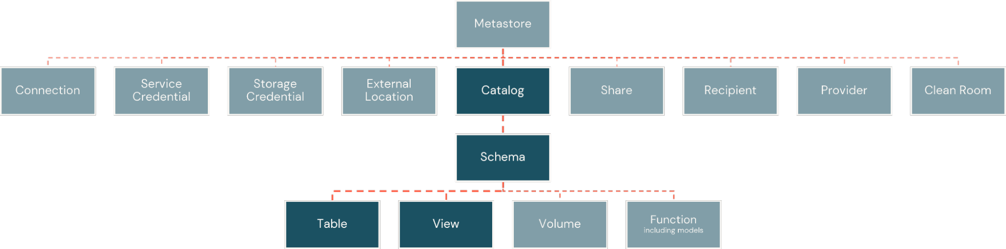
Within the Databricks Platform, facts and dimensions are implemented as physical tables. These are organized within catalogs, similar to databases, but with greater flexibility for the breadth of information assets the platform supports. The catalogs are then subdivided into schemas, creating logical and security boundaries around subsets of objects in the catalog (Figure 2).
Dimension tables
Dimension tables adhere to a relatively rigid set of structural patterns. A sequential identifier, a surrogate key, is typically defined to support a stable and efficient linkage between fact tables and the dimension. Unique identifiers from operational systems (often referred to as natural keys or business keys), along with a denormalized collection of related business attributes, typically follow. Behind the identifiers are usually a series of metadata columns intended to support ongoing ETL processes. Within the Databricks Platform, we can implement a dimension table using the CREATE TABLE statement, as is shown here for the customer dimension:
Identity columns
In this example, for the surrogate key column, CustomerKey, we employ an identity column that automatically creates a sequential BIGINT value for the field as we insert rows. Whether we use the ALWAYS or BY DEFAULT option with the identity column depends on whether we want to prohibit or permit the insertion of our own values for this field.
Missing member entry
A common pattern implemented with dimension tables is creating a missing member entry. This entry is used in scenarios where fact records arrive with missing or unknown linkage to a dimension and can be created with a pre-determined surrogate key value like what is shown here when the BY DEFAULT option is employed:
Identity fields
As a best practice, whenever inserting values into an identify field, it is best to ensure the metadata for the identify field is updated through the use of an ALTER TABLE statement with the SYNC IDENTITY option employed:
Data types
For the business/natural key and other fields tied to data in source systems, we will need to align source system data types with those data types supported by the Databricks Platform (Table 1). For metadata fields where a bit value is employed, like 0 or 1, please note that we often use an INT data type instead of the BOOLEAN or TINYINT data types to make handling literals a bit easier.
|
BIGINT |
DECIMAL |
INTERVAL |
TIMESTAMP |
MAP |
|
BINARY |
DOUBLE |
VOID |
TIMESTAMP_NTZ |
STRUCT |
|
BOOLEAN |
FLOAT |
SMALLINT |
TINYINT |
VARIANT |
|
DATE |
INT |
STRING |
ARRAY |
OBJECT |
Table 1. The data types supported by the Databricks Platform
Fact tables
Fact tables, too, follow their structural conventions. Composed primarily of measures and foreign key references to related dimensions, fact tables may also include unique identifiers for transactional records (or other descriptive attributes in a nearly one-to-one relationship with the fact records), referred to as degenerate dimensions. They may also include metadata fields to support the incremental loading (aka delta extract) of data from source systems. Within the Databricks Platform, we might implement a fact table using the CREATE TABLE statement similar to what is shown here for the Internet sales fact:
Foreign key references
As mentioned in the previous section on dimension tables, data types in the Databricks environment are loosely mapped to those employed by source systems. The foreign key references between the fact and dimension tables can also be made explicit using the ALTER TABLE statement as shown here:
Note: If you prefer to define the foreign key constraints as part of the CREATE TABLE statement, you can simply add a comma-separated list of FOREIGN KEY clauses (in the form FOREIGN KEY (foreign_key) REFERENCES table_name (primary_key) just after the column-definition list.
Metadata and other considerations
The appeal of the dimensional model is its relative accessibility to business analysts. With this in mind, many organizations adopt naming conventions for facts and dimensions, such as the Fact and Dim prefixes in the examples above, and encourage using long, self-explanatory names for tables and fields that often deviate significantly from the names employed in operational source systems.
With this in mind, it’s important to note the limitations of Databricks on naming objects. These include:
- Object names cannot exceed 255 characters
- The following special characters are not allowed:
- Period (.)
- Space ( )
- Forward slash (/)
- All ASCII control characters (00-1F hex)
- The DELETE character (7F hex)
In addition, it’s important to note that object names are not case sensitive and are, in fact, stored in the metadata repository in all lowercase. If this might create problems with object readability, you might consider adopting a snake case convention to improve the readability of some object names.
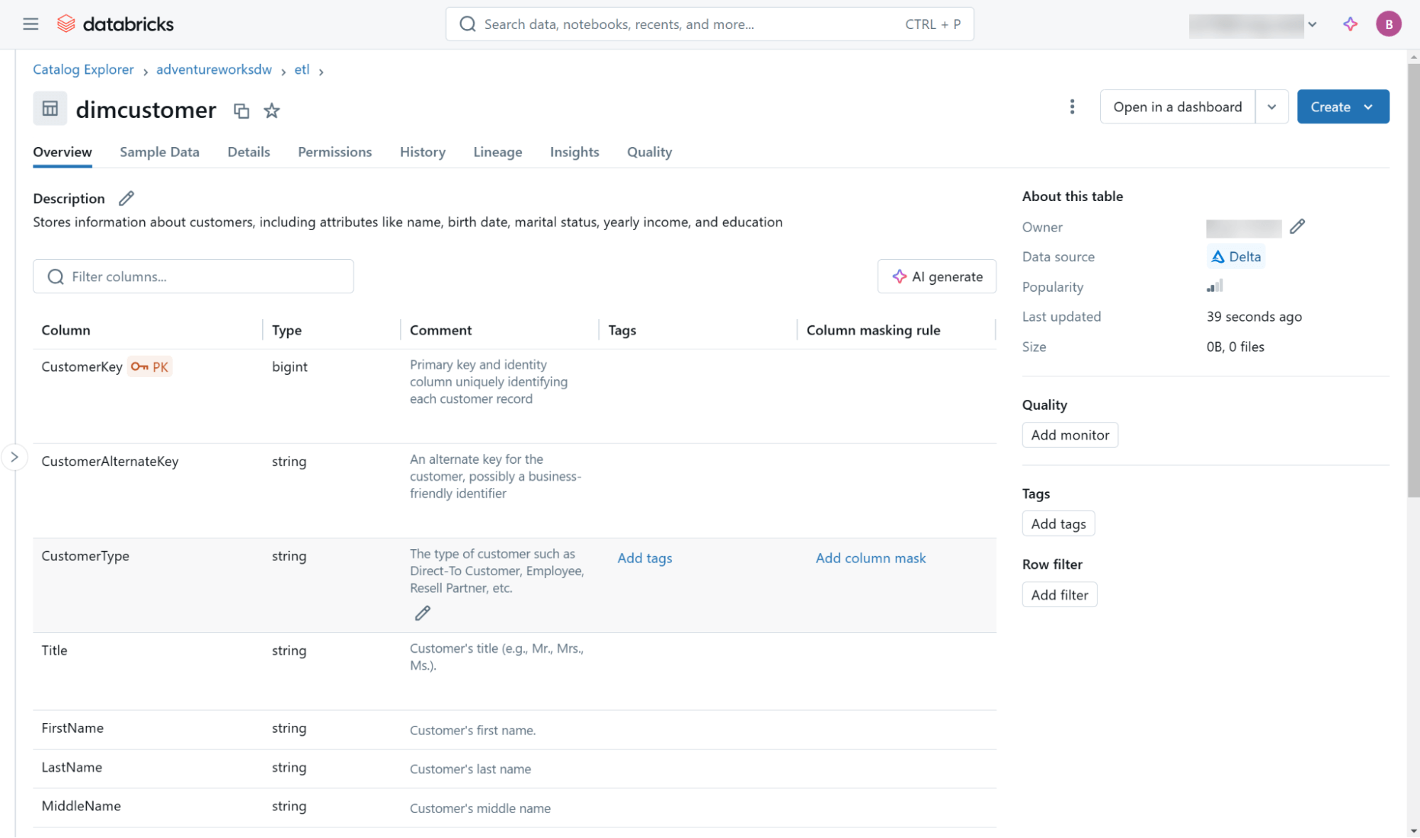
Regardless of your naming conventions, it’s a good idea to define descriptive comments for all objects and fields within the data warehouse. This is done through the use of COMMENT ON statement for table objects and the ALTER TABLE statement for individual fields, as demonstrated here:
This and other metadata (including lineage information) are accessible through the Databricks Catalog Explorer user interface (Figure 3) and through objects in the built-in information schema found within each catalog.
Lastly, this blog addresses the creation of fact and dimension tables purely from the perspective of adhering to dimensional design principles. If you’d like to explore some additional options for table definition that consider performance and maintenance optimizations, please check out this blog on optimizing star schema performance.
Next steps: implementing the dimension table ETL
After addressing the basics behind fact and dimension table creation, we will turn our attention in the next blog to implementing the ETL patterns supporting dimension tables, with a special emphasis on the Type-1 and Type-2 slowly changing dimension (SCD) patterns using both Python and SQL. Finally, Part 3 will cover how the ETL for these tables can be implemented.
To learn more about Databricks SQL, visit our website or read the documentation. You can also check out the product tour for Databricks SQL. Suppose you want to migrate your existing warehouse to a high-performance, serverless data warehouse with a great user experience and lower total cost. In that case, Databricks SQL is the solution — try it for free.

