Tuning Java Garbage Collection for Apache Spark Applications

This is a guest post from our friends in the SSG STO Big Data Technology group at Intel.

Join us at the Spark Summit to hear from Intel and other companies deploying Apache Spark in production.  Use the code Databricks20 to receive a 20% discount!

Apache Spark is gaining wide industry adoption due to its superior performance, simple interfaces, and a rich library for analysis and calculation. Like many projects in the big data ecosystem, Spark runs on the Java Virtual Machine (JVM). Because Spark can store large amounts of data in memory, it has a major reliance on Java's memory management and garbage collection (GC). New initiatives like Project Tungsten will simplify and optimize memory management in future Spark versions. But today, users who understand Java's GC options and parameters can tune them to eek out the best the performance of their Spark applications. This article describes how to configure the JVM's garbage collector for Spark, and gives actual use cases that explain how to tune GC in order to improve Spark's performance. We look at key considerations when tuning GC, such as collection throughput and latency.

Introduction to Spark and Garbage Collection

With Spark being widely used in industry, Spark applications' stability and performance tuning issues are increasingly a topic of interest. Due to Spark's memory-centric approach, it is common to use 100GB or more memory as heap space, which is rarely seen in traditional Java applications. In working with large companies using Spark, we receive plenty of concerns about the various challenges surrounding GC during execution of Spark applications. For example, garbage collection takes a long time, causing program to experience long delays, or even crash in severe cases. In this article, we use real examples, combined with the specific issues, to discuss GC tuning methods for Spark applications that can alleviate these problems.

Java applications typically use one of two garbage collection strategies: Concurrent Mark Sweep (CMS) garbage collection and ParallelOld garbage collection. The former aims at lower latency, while the latter is targeted for higher throughput. Both strategies have performance bottlenecks: CMS GC does not do compaction[1], while Parallel GC performs only whole-heap compaction, which results in considerable pause times. At Intel, we advise our customers to choose the strategy which best suits a given application's requirements. For applications with real-time response, we generally recommend CMS GC; for off-line analysis programs, we use Parallel GC.

So for a computing framework such as Spark that supports both streaming computing and traditional batch processing, can we find an optimal collector? The Hotspot JVM version 1.6 introduced a third option for garbage collections: the Garbage-First GC (G1 GC). The G1 collector is planned by Oracle as the long term replacement for the CMS GC. Most importantly, the G1 collector aims to achieve both high throughput and low latency. Before we go into details on using the G1 collector with Spark, let's go over some background on Java GC fundamentals.

How Java's Garbage Collectors Work

In traditional JVM memory management, heap space is divided into Young and Old generations. The young generation consists of an area called Eden along with two smaller survivor spaces, as shown in Figure 1. Newly created objects are initially allocated in Eden. Each time a minor GC occurs, the JVM copies live objects in Eden to an empty survivor space and also copies live objects in the other survivor space that is being used to that empty survivor space. This approach leaves one of the survivor spaces holding objects, and the other empty for the next collection. Objects that have survived some number of minor collections will be copied to the old generation. When the old generation fills up, a major GC will suspend all threads to perform full GC, namely organizing or removing objects in the old generation. This execution pause when all threads are suspended is called Stop-The-World (STW), which sacrifices performance in most GC algorithms. [2]

Figure 1 Generational Hotspot Heap Structure [2] **

Java's newer G1 GC completely changes the traditional approach. The heap is partitioned into a set of equal-sized heap regions, each a contiguous range of virtual memory (Figure 2). Certain region sets are assigned the same roles (Eden, survivor, old) as in the older collectors, but there is not a fixed size for them. This provides greater flexibility in memory usage. When an object is created, it is initially allocated in an available region. When the region fills up, JVM creates new regions to store objects. When minor GC occurs, G1 copies live objects from one or more regions of the heap to a single region on the heap, and select a few free new regions as Eden regions. Full GC occurs only when all regions hold live objects and no full-empty region can be found. G1 uses the Remembered Sets (RSets) concept when marking live objects. RSets track object references into a given region by external regions. There is one RSet per region in the heap. The RSet avoids whole-heap scan, and enables the parallel and independent collection of a region. In this context, we can see that G1 GC not only greatly improves heap occupancy rate when full GC is triggered, but also makes the minor GC pause times more controllable, thereby is very friendly for large memory environment. How do these disruptive improvements change GC performance? Here we use the easiest way to observe the performance changes, i.e. by migrating from old GC settings to G1 GC settings. [3]

Figure 2 Illustration for G1 Heap Structure [3]**

Since G1 gives up the approach of using fixed heap partitions for young/aged objects, we have to adjust GC configuration options accordingly to safeguard the smooth running of the application with G1 collector. Unlike with older garbage collectors, we've generally found that a good starting point with the G1 collector is not to perform any tuning. So we recommend beginning only with the default settings and simply enabling G1 via the -XX:+UseG1GC option. One tweak we have found sometimes useful is that, when an application uses multiple threads, it is best to use -XX: -ResizePLAB to close PLAB() resize and avoid performance degradation caused by a large number of thread communications.

For a complete list of GC parameters supported by Hotspot JVM, you can use the parameter -XX: +PrintFlagsFinal to print out the list, or refer to the Oracle official documentation for explanations on part of the parameters.

Understanding Memory Management in Spark

A Resilient Distributed Dataset (RDD) is the core abstraction in Spark. Creation and caching of RDD's closely related to memory consumption. Spark allows users to persistently cache data for reuse in applications, thereby avoid the overhead caused by repeated computing. One form of persisting RDD is to cache all or part of the data in JVM heap. Spark's executors divide JVM heap space into two fractions: one fraction is used to store data persistently cached into memory by Spark application; the remaining fraction is used as JVM heap space, responsible for memory consumption during RDD transformation. We can adjust the ratio of these two fractions using the spark.storage.memoryFraction parameter to let Spark control the total size of the cached RDD by making sure it doesn't exceed RDD heap space volume multiplied by this parameter's value. The unused portion of the RDD cache fraction can also be used by JVM. Therefore, GC analysis for Spark applications should cover memory usage of both memory fractions.

When an efficiency decline caused by GC latency is observed, we should first check and make sure the Spark application uses the limited memory space in an effective way. The less memory space RDD takes up, the more heap space is left for program execution, which increases GC efficiency; on the contrary, excessive memory consumption by RDDs leads to significant performance loss due to a large number of buffered objects in the old generation. Here we expand on this point with a use case:

For example, the user has an application based on the Bagel component of Spark, which performs simple iterative computing. The result of one superstep (iteration) depends on that of the previous superstep, so the result of each superstep will be persisted in memory space. During program execution, we observed that when the number of iterations increase, the memory space used by progress grows rapidly, causing GC to get worse. When we looked closely at Bagel, we discovered that it caches the RDDs of each superstep in memory without freeing them up over time, even though they are not used after a single iteration. This leads to a memory consumption growth that triggers more GC attempts. We removed this unnecessary caching in SPARK-2661. After this modification cache, RDD size stabilizes after three iterations and cache space is now effectively controlled (as shown in Table 1). As a result, GC efficiency has been greatly improved, with the total running time of the program shortened by 10%~20%.

Table 1: Comparison of Bagel Application's RDD Cache Sizes before and after Optimization

Conclusion:

When GC is observed as too frequent or long lasting, it may indicate that memory space is not used efficiently by Spark process or application. You can improve performance by explicitly cleaning up cached RDD's after they are no longer needed.

Choosing a Garbage Collector

If our application is using memory as efficiently as possible, the next step is to tune our choice of garbage collector. After implementing SPARK-2661, we set up a four-node cluster, assigned an 88GB heap to each executor, and launched Spark in Standalone mode to conduct our experiments. We started with the default Spark Parallel GC, and found that because the Spark application's memory overhead is relatively large and most of the objects cannot be reclaimed in a reasonably short life cycle, the Parallel GC is often trapped in full GC, which brings a decline to performance every time it occurs. To make it worse, Parallel GC provides very limited options for performance tuning, so we can only use some basic parameters to adjust performance, such as the size ratio of each generation, and the number of copies before objects are promoted to the old generation. Since these tuning strategies only postpone full GC, the Parallel GC tuning helps little to long-running applications. Therefore, in this article we do not proceed with the Parallel GC tuning. Table 2 shows the operation of the Parallel GC, and obviously when the full GC is executed the lowest CPU utilization rates occur.

Table 2: Parallel GC Running Status (Before Tuning)

Configuration Options	-XX:+UseParallelGC -XX:+UseParallelOldGC -XX:+PrintFlagsFinal -XX:+PrintReferenceGC -verbose:gc -XX:+PrintGCDetails -XX:+PrintGCTimeStamps -XX:+PrintAdaptiveSizePolicy -Xms88g -Xmx88g
Stage*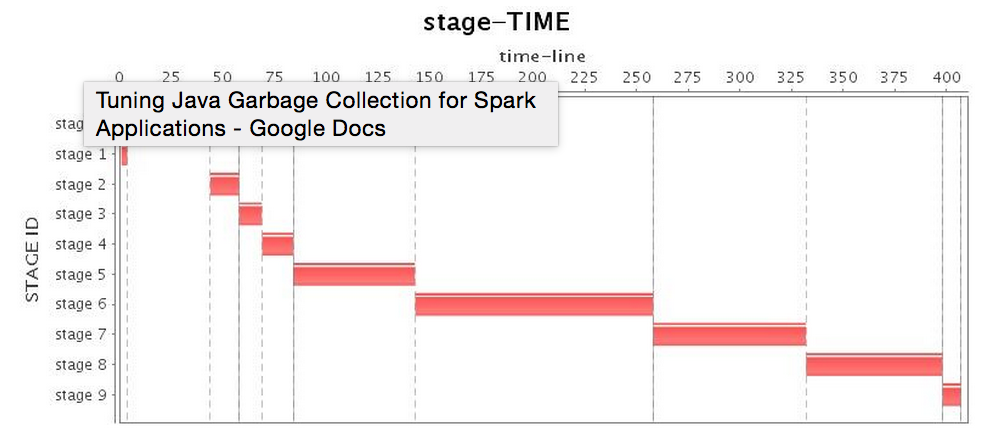
Task*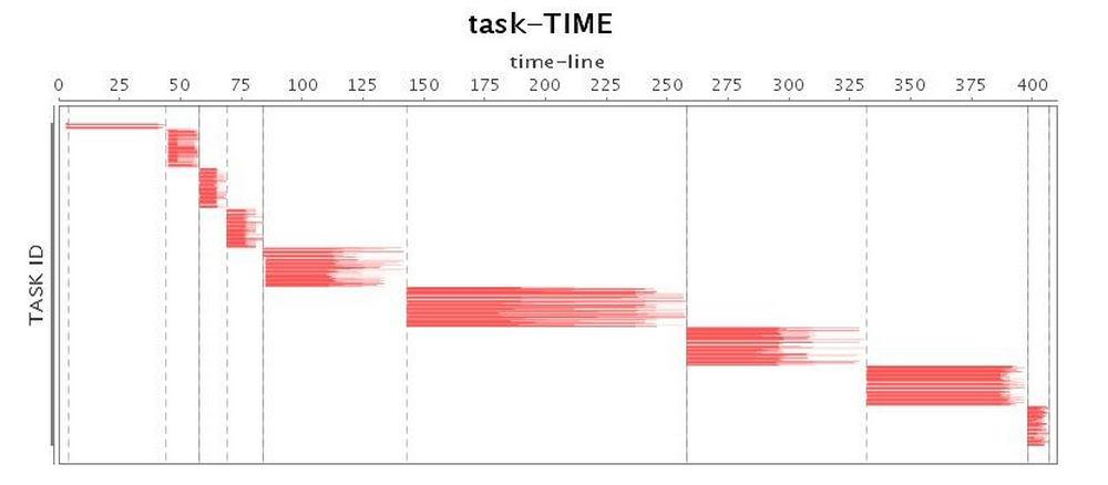
CPU*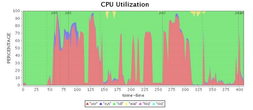
Mem*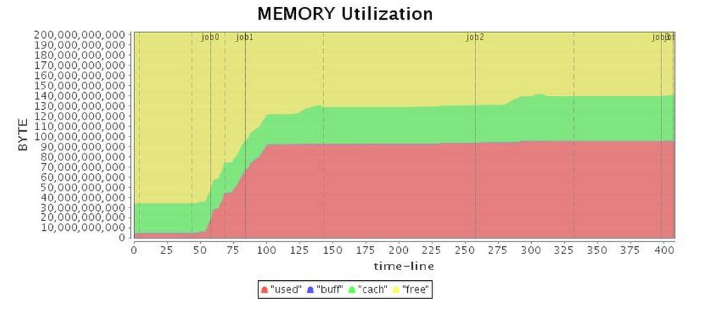

CMS GC cannot do anything to eliminate full GC in this Spark application. Moreover, CMS GC has much longer full GC pause times than Parallel GC, taking a big bite out of the application's throughput.

Next, we ran our application with default G1 GC configuration. To our surprise, G1 GC also gave unacceptable full GC (see "CPU Utilization" in Table 3, obviously Job 3 paused nearly 100 seconds), and a long pause time significantly dragged down the entire application operation. As shown in Table 4, although the total running time is slightly longer than the Parallel GC, G1 GC's performance was slightly better than the CMS GC.

Table 3: G1 GC Running Status (Before Tuning)

Configuration Options	-XX:+UseG1GC -XX:+PrintFlagsFinal -XX:+PrintReferenceGC -verbose:gc -XX:+PrintGCDetails -XX:+PrintGCTimeStamps -XX:+PrintAdaptiveSizePolicy -XX:+UnlockDiagnosticVMOptions -XX:+G1SummarizeConcMark -Xms88g -Xmx88g
Stage*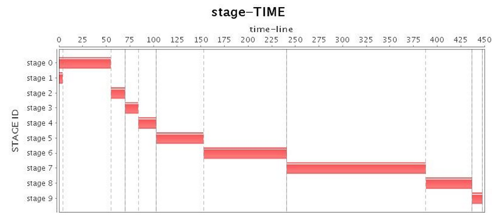
Task*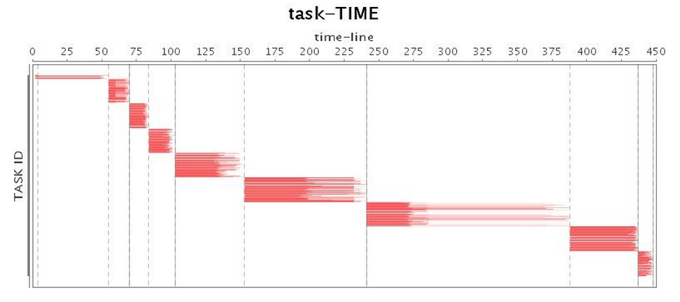
CPU*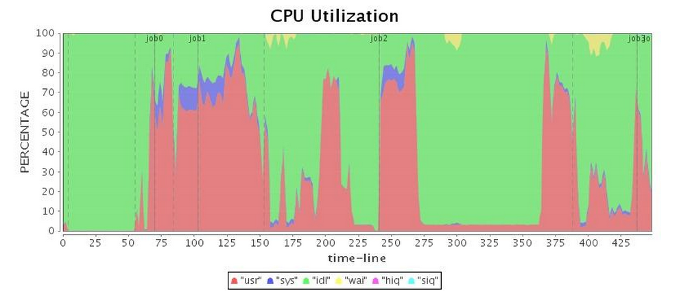
Mem*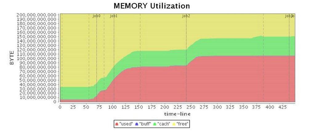

Table 4 Comparison of Three Garbage Collectors' Program Running Time (88GB Heap before tuning)

Tuning The G1 Collector Based on Logs[4][5]

After we set up G1 GC, the next step is to further tune the collector performance based on GC log.

First of all, we want JVM to record more details in GC log. So for Spark, we set "spark.executor.extraJavaOptions" to include additional flags. In general, we need to set such options:

-XX:+PrintFlagsFinal -XX:+PrintReferenceGC -verbose:gc -XX:+PrintGCDetails -XX:+PrintGCTimeStamps -XX:+PrintAdaptiveSizePolicy -XX:+UnlockDiagnosticVMOptions -XX:+G1SummarizeConcMark

With these options defined, we keep track of detailed GC log and effective GC options in Spark's executer log (output to $SPARK_HOME/work/$ app_id/$executor_id/stdout at each worker node). Next, we can analyze root cause of the problems according to GC log and learn how to improve the program performance.

Let's take a look at the structure of a G1 GC log as follows, which takes a mixed GC in G1 GC for example.

251.354: [G1Ergonomics (Mixed GCs) continue mixed GCs, reason: candidate old regions available, candidate old regions: 363 regions, reclaimable: 9830652576 bytes (10.40 %), threshold: 10.00 %]

[Parallel Time: 145.1 ms, GC Workers: 23]

[GC Worker Start (ms): Min: 251176.0, Avg: 251176.4, Max: 251176.7, Diff: 0.7]

[Ext Root Scanning (ms): Min: 0.8, Avg: 1.2, Max: 1.7, Diff: 0.9, Sum: 28.1]

[Update RS (ms): Min: 0.0, Avg: 0.3, Max: 0.6, Diff: 0.6, Sum: 5.8]

[Processed Buffers: Min: 0, Avg: 1.6, Max: 9, Diff: 9, Sum: 37]

[Scan RS (ms): Min: 6.0, Avg: 6.2, Max: 6.3, Diff: 0.3, Sum: 143.0]

[Object Copy (ms): Min: 136.2, Avg: 136.3, Max: 136.4, Diff: 0.3, Sum: 3133.9]

[Termination (ms): Min: 0.0, Avg: 0.0, Max: 0.0, Diff: 0.0, Sum: 0.3]

[GC Worker Other (ms): Min: 0.0, Avg: 0.1, Max: 0.2, Diff: 0.2, Sum: 1.9]

[GC Worker Total (ms): Min: 143.7, Avg: 144.0, Max: 144.5, Diff: 0.8, Sum: 3313.0]

[GC Worker End (ms): Min: 251320.4, Avg: 251320.5, Max: 251320.6, Diff: 0.2]

[Code Root Fixup: 0.0 ms]

[Clear CT: 6.6 ms]

[Other: 26.8 ms]

[Choose CSet: 0.2 ms]

[Ref Proc: 16.6 ms]

[Ref Enq: 0.9 ms]

[Free CSet: 2.0 ms]

[Eden: 3904.0M(3904.0M)->0.0B(4448.0M) Survivors: 576.0M->32.0M Heap: 63.7G(88.0G)->58.3G(88.0G)]

[Times: user=3.43 sys=0.01, real=0.18 secs]

From this log, we can see that G1 GC log has a very clear hierarchy. The log lists when and why the pause occurs, and grades time consumption of various threads as well as average and maximum CPU time. Finally, G1 GC lists the cleanup results after this pause, and the total time consumption.

In our current G1 GC running log, we find a special block like this:

(to-space exhausted), 1.0552680 secs]

[Parallel Time: 958.8 ms, GC Workers: 23]

[GC Worker Start (ms): Min: 759925.0, Avg: 759925.1, Max: 759925.3, Diff: 0.3]

[Ext Root Scanning (ms): Min: 1.1, Avg: 1.4, Max: 1.8, Diff: 0.6, Sum: 33.0]

[SATB Filtering (ms): Min: 0.0, Avg: 0.0, Max: 0.3, Diff: 0.3, Sum: 0.3]

[Update RS (ms): Min: 0.0, Avg: 1.2, Max: 2.1, Diff: 2.1, Sum: 26.9]

[Processed Buffers: Min: 0, Avg: 2.8, Max: 11, Diff: 11, Sum: 65]

[Scan RS (ms): Min: 1.6, Avg: 2.5, Max: 3.0, Diff: 1.4, Sum: 58.0]

[Object Copy (ms): Min: 952.5, Avg: 953.0, Max: 954.3, Diff: 1.7, Sum: 21919.4]

[Termination (ms): Min: 0.0, Avg: 0.1, Max: 0.2, Diff: 0.2, Sum: 2.2]

[GC Worker Other (ms): Min: 0.0, Avg: 0.0, Max: 0.0, Diff: 0.0, Sum: 0.6]

[GC Worker Total (ms): Min: 958.1, Avg: 958.3, Max: 958.4, Diff: 0.3, Sum: 22040.4]

[GC Worker End (ms): Min: 760883.4, Avg: 760883.4, Max: 760883.4, Diff: 0.0]

[Code Root Fixup: 0.0 ms]

[Clear CT: 0.4 ms]

[Other: 96.0 ms]

[Choose CSet: 0.0 ms]

[Ref Proc: 0.4 ms]

[Ref Enq: 0.0 ms]

[Free CSet: 0.1 ms]

[Eden: 160.0M(3904.0M)->0.0B(4480.0M) Survivors: 576.0M->0.0B Heap: 87.7G(88.0G)->87.7G(88.0G)]

[Times: user=1.69 sys=0.24, real=1.05 secs]

760.981: [G1Ergonomics (Heap Sizing) attempt heap expansion, reason: allocation request failed, allocation request: 90128 bytes]

760.981: [G1Ergonomics (Heap Sizing) expand the heap, requested expansion amount: 33554432 bytes, attempted expansion amount: 33554432 bytes]

760.981: [G1Ergonomics (Heap Sizing) did not expand the heap, reason: heap expansion operation failed]

760.981: [Full GC 87G->36G(88G), 67.4381220 secs]

As we can see, the largest performance degradation was caused by such a full GC, and was output in the log as To-space Exhausted, To-space Overflow or the similar (for various JVM versions, the output may look slightly different). The cause is that when the G1 GC collector tries to collect garbage for certain regions, it fails to find free regions which it can copy the live objects to. This situation is called Evacuation Failure and often leads to full GC. And apparently, full GC in G1 GC is even worse than in Parallel GC, so we must try to avoid full GC in order to achieve better performance. To avoid full GC in G1 GC, there are two commonly-used approaches:

1. Decrease the InitiatingHeapOccupancyPercent option's value (the default value is 45), to let G1 GC starts initial concurrent marking at an earlier time, so that we are more likely to avoid full GC.
2. Increase the ConcGCThreads option's value, to have more threads for concurrent marking, thus we can speed up the concurrent marking phase. Take caution that this option could also take up some effective worker thread resources, depending on your workload CPU utilization.

Tuning these two options minimized the possibility of a full GC occurrences. After full GC was eliminated, performance was increased dramatically. However, we still found long pauses during GC. On further investigation, we found the following occurrence in our logs:

280.008: [G1Ergonomics (Concurrent Cycles) request concurrent cycle initiation, reason: occupancy higher than threshold, occupancy: 62344134656 bytes, allocation request: 46137368 bytes, threshold: 42520176225 bytes (45.00 %), source: concurrent humongous allocation]

Here we see humongous objects (objects that are 50% the size of a standard region or larger). G1 GC would put each of these objects in contiguous set of regions. And since copying these objects would consume a lot of resources, humongous objects are directly allocated out of the old generation (bypassing all young GCs) and then categorized into humongous regions [4]. Before 1.8.0_u40, a complete heap liveness analysis is required to reclaim humongous regions [JDK-8027959]. If there are many objects of this kind, the heap would be filled up very quickly, and to reclaim them is too expensive. Even with the fixes (they do increase the efficiency of reclaiming humongous objects greatly), the allocation of contiguous regions is still more expensive (especially when meeting serious heap fragmentations), so we want to avoid creating objects of this size. We can increase the value of G1HeapRegionSize to reduce possibility of creating humongous regions, but the default value is already at its maximum size of 32M if we are using a comparatively large heap. This means we can only analyze the program to find these objects and to minimize their creation. Otherwise, it likely leads to more concurrent marking phase, and after that, you need to carefully tune mix GC related knobs (e.g., -XX:G1HeapWastePercent -XX:G1MixedGCLiveThresholdPercent) to avoid long mix GC pauses (caused by lots of humongous objects).

Next, we can analyze the interval of a single GC cycle from cycle start until end of mixed GC. If the time is too long, you can consider increasing the value of ConcGCThreads, but note that this will take up more CPU resources.

The G1 GC also has ways to decrease STW pause length in return for doing more work in the concurrent stage of garbage collection. As mentioned above, G1 GC maintains an Remembered Set(RSet) for each region to track object references into a given region by external regions, and G1 collector updates RSets both at the STW stage and at the concurrent stage. If you are seeking to decrease the length of STW pauses with the G1 GC, you can decrease the value of G1RSetUpdatingPauseTimePercent while increasing the value of G1ConcRefinementThreads. The option G1RSetUpdatingPauseTimePercent is used to specify a desired ratio of RSets update time in total STW time, which is 10-percent by default, and G1ConcRefinementThreads is used to define the number of threads for maintaining RSets during program running. With these two options tuned, we can shift more workloads of RSets updating from STW stage to concurrent stage.

In addition, for long-running applications, we use the AlwaysPreTouch option, so JVM applies all the memory needed to OS at startup and avoids dynamic applications. This improves runtime performance at the cost of extending the start time.

Eventually, after several rounds of GC parameters tuning, we arrived at the results in Table 5. Compared with the previous results, we finally obtained a more satisfactory running efficiency.

Table 5 G1 GC Running Status (after Tuning)

Configuration Options	-XX:+UseG1GC -XX:+PrintFlagsFinal -XX:+PrintReferenceGC -verbose:gc -XX:+PrintGCDetails -XX:+PrintGCTimeStamps -XX:+PrintAdaptiveSizePolicy -XX:+UnlockDiagnosticVMOptions -XX:+G1SummarizeConcMark -Xms88g -Xmx88g -XX:InitiatingHeapOccupancyPercent=35 -XX:ConcGCThread=20
Stage*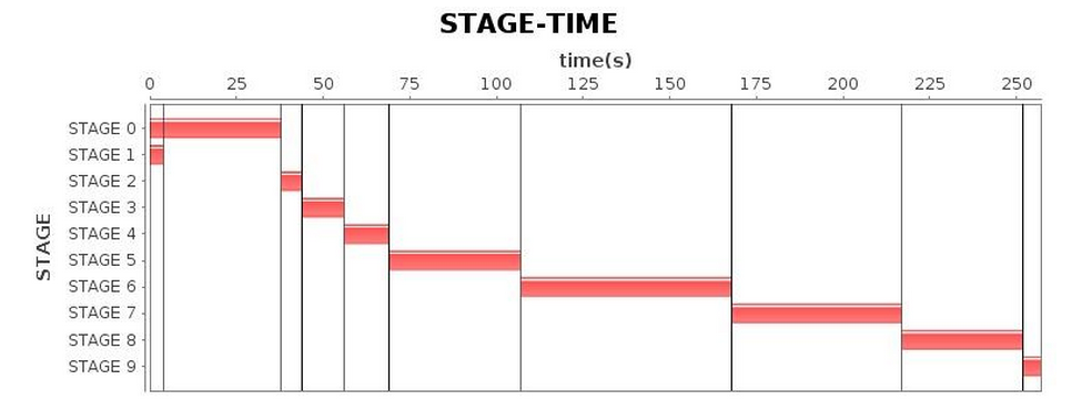
Task*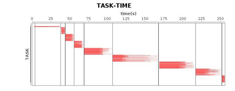
CPU*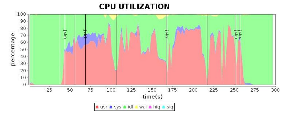
Mem*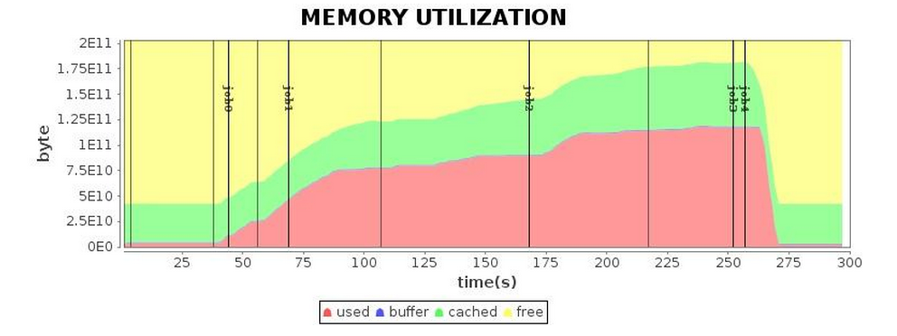

Conclusion:

We recommend trying the G1 GC compared with alternatives for Spark applications. Finer-grained optimizations can be obtained through GC log analysis. After tuning, we successfully shortened the running time of the application to 4.3 minutes. Compared with the running time before tuning, we achieved a performance increase of 1.7 times; compared with Parallel GC, an increase by 1.5 times more or less.

Summary

For Spark applications which rely heavily on memory computing, GC tuning is particularly important. When problems emerge with GC, do not rush into debugging the GC itself. First consider inefficiency in Spark program's memory management, such as persisting and freeing up RDD in cache. When tuning garbage collectors, we first recommend using G1 GC to run Spark applications. The G1 collector is well poised to handle growing heap sizes often seen with Spark. With G1, fewer options will be needed to provide both higher throughput and lower latency. Of course, there is no fixed pattern for GC tuning. The various applications have different characteristics, and in order to tackle unpredictable situations, one must master the art of GC tuning according to logs and other forensics. Finally, we cannot forget optimizing through program's logic and code, such as reducing intermediate object creation or replication, controlling creation of large objects, storing long-lived objects in off-heap, and so on.

By using the G1 GC we achieved major performance improvements in Spark applications. Future work in Spark will move memory management responsibility away from Java's garbage collectors and into Spark itself. This will alleviate much of the tuning requirements for Spark applications. Nonetheless, today garbage collector choice can increase performance for mission critical Spark applications.

Acknowledgement

During the tuning practice and writing of this article, we received guidance and assistance from Ms. Yanping Wang, senior engineer from Intel's Java Runtime team.

* Indicates graphs generated using internal Performance Analysis tools developed by Intel Big Data team.

** Indicates images from Oracle documentation. For details, see reference [2] [3]

References

1. https://docs.oracle.com/cd/E13150_01/jrockit_jvm/jrockit/geninfo/diagnos/garbage_collect.html#wp1086917
2. https://www.oracle.com/webfolder/technetwork/tutorials/obe/java/gc01/index.html
3. https://www.oracle.com/webfolder/technetwork/tutorials/obe/java/G1GettingStarted/index.html
4. https://www.infoq.com/articles/tuning-tips-G1-GC/
5. https://blogs.oracle.com/

About the Authors:

Daoyuan Wang, Software Engineer from SSG STO Big Data Technology, Intel Asia-Pacific Research & Development Ltd., who is also an active Spark contributor in the Apache community.

Jie Huang, engineering manager of SSG STO Big Data Technology, Intel Asia-Pacific Research & Development Ltd.