A Convolutional Neural Network Implementation For Car Classification
by Dr. Evan Eames and Henning Kropp
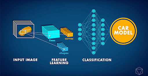
Convolutional Neural Networks (CNN) are state-of-the-art Neural Network architectures that are primarily used for computer vision tasks. CNN can be applied to a number of different tasks, such as image recognition, object localization, and change detection. Recently, our partner Data Insights received a challenging request from a major car company: Develop a Computer Vision application which could identify the car model in a given image. Considering that different car models can appear quite similar and any car can look very different depending on their surroundings and the angle at which they are photographed, such a task was, until quite recently, simply impossible.

However, starting around 2012, the ‘Deep Learning Revolution’ made it possible to handle such a problem. Instead of being explained the concept of a car, computers could instead repeatedly study pictures and learn such concepts themselves. In the past few years, additional Artificial Neural Network innovations have resulted in AI that can perform image classification tasks with human-level accuracy. Building on such developments we were able to train a Deep CNN to classify cars by their model. The Neural Network was trained on the Stanford Cars Dataset, which contains over 16,000 pictures of cars, comprising 196 different models. Over time we could see the accuracy of predictions began to improve, as the neural network learned the concept of a car, and how to distinguish between different models.
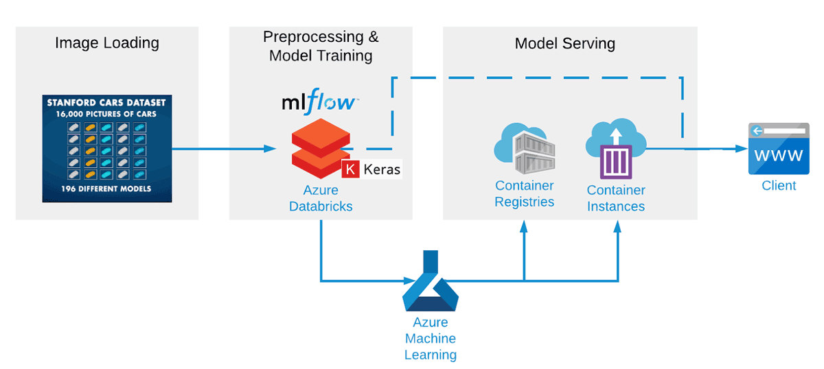
Together with our partner we build an end-to-end machine learning pipeline using Apache Spark™ and Koalas for the data preprocessing, Keras with Tensorflow for the model training, MLflow for the tracking of models and results, and Azure ML for the deployment of a REST service. This setup within Azure Databricks is optimized to train networks fast and efficiently, and also helps to try many different CNN configurations much more quickly. Even after only a few practice attempts, the CNN's accuracy reached around 85%.
Setting up an Artificial Neural Network to Classify Images
In this article we are outlining some of the main techniques used in getting a Neural Network up into production. If you’d like to attempt to get the Neural Network running yourself, the full notebooks with a meticulous step-by-step guide included, can be found below.
This demo uses the publicly available Stanford Cars Dataset which is one of the more comprehensive public data sets, although a little outdated, so you won’t find car models post 2012 (although, once trained, transfer learning could easily allow a new dataset to be substituted). The data is provided through an ADLS Gen2 storage account that you can mount to your workspace.

For the first step of data preprocessing the images are compressed into hdf5 files (one for training and one for testing). This can then be read in by the neural network. This step can be omitted completely, if you like, as the hdf5 files are part of the ADLS Gen2 storage provided as part of the here provided notebooks.
- Load Stanford Cars dataset into HDF5 files
- Use Koalas for image augmentation
- Train the CNN with Keras
- Deploy model as REST service to Azure ML
Image Augmentation with Koalas
The quantity and diversity of data gathered has a large impact on the results one can achieve with deep learning models. Data augmentation is a strategy that can significantly improve learning results without the need to actually collect new data. With different techniques like cropping, padding, and horizontal flipping, which are commonly used to train large neural networks, the data sets can be artificially inflated by increasing the number of images for training and testing.
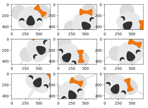
Applying augmentation to a large corpus of training data can be very expensive, especially when comparing the results of different approaches. With Koalas it becomes easy to try existing frameworks for image augmentation in Python, and scaling the process out on a cluster with multiple nodes using the to data science familiar Pandas API.
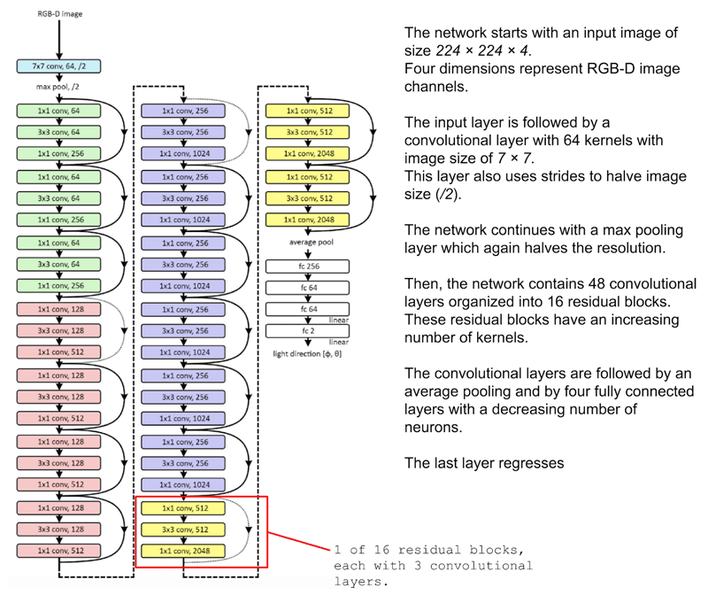
Coding a ResNet in Keras
When you break apart a CNN, they comprise different ‘blocks’, with each block simply representing a group of operations to be applied to some input data. These blocks can be broadly categorized into:
- Identity Block: A series of operations which keep the shape of the data the same.
- Convolution Block: A series of operations which reduce the shape of the input data to a smaller shape.
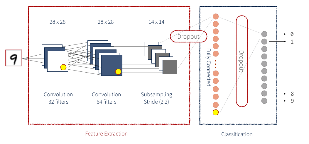
A CNN is a series of both Identity Blocks and Convolution Blocks (or ConvBlocks) which reduce an input image to a compact group of numbers. Each of these resulting numbers (if trained correctly) should eventually tell you something useful towards classifying the image. A Residual CNN adds an additional step for each block. The data is saved as a temporary variable before the operations that constitute the block are applied, and then this temporary data is added to the output data. Generally, this additional step is applied to each block. As an example the below figure demonstrates a simplified CNN for detecting handwritten numbers:
There are many different methods of implementing a Neural Network. One of the more intuitive ways is via Keras. Keras provides a simple front-end library for executing the individual steps which comprise a neural network. Keras can be configured to work with a Tensorflow back-end, or a Theano back-end. Here, we will be using a Tensorflow back-end. A Keras network is broken up into multiple layers as seen below. For our network we are also defining our customer implementation of a layer.
The Scale Layer
For any custom operation that has trainable weights Keras allows you to implement your own layer. When dealing with huge amounts of image data, one can run into memory issues. Initially, RGB images contain integer data (0-255). When running gradient descent as part of the optimisation during backpropagation, one will find that integer gradients do not allow for sufficient accuracy to properly adjust network weights. Therefore, it is necessary to change to float precision. This is where issues can arise. Even when images are scaled down to 224x224x3, when we use ten thousand training images, we are looking at over 1 billion floating point entries. As opposed to turning an entire dataset to float precision, better practice is to use a ‘Scale Layer’, which scales the input data one image at a time, and only when it is needed. This should be applied after Batch Normalization in the model. The parameters of this Scale Layer are also parameters that can be learned through training.
To use this custom layer also during scoring we have to package the class together with our model. With MLflow we can achieve this with a Keras custom_objects dictionary mapping names (strings) to custom classes or functions associated with the Keras model. MLflow saves these custom layers using CloudPickle and restores them automatically when the model is loaded with mlflow.keras.load_model() and mlflow.pyfunc.load_model().
Tracking Results with MLflow and Azure Machine Learning
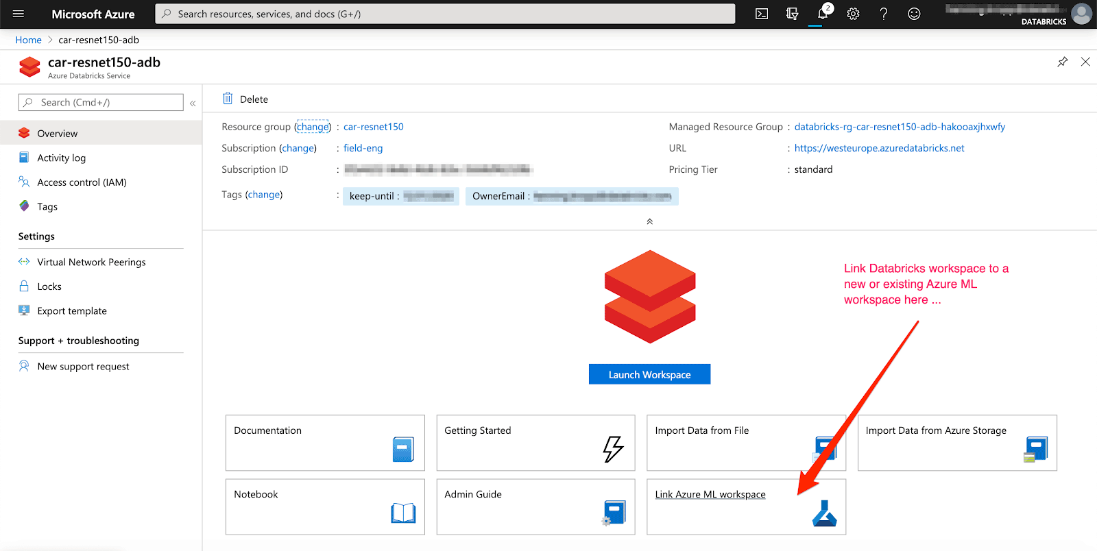
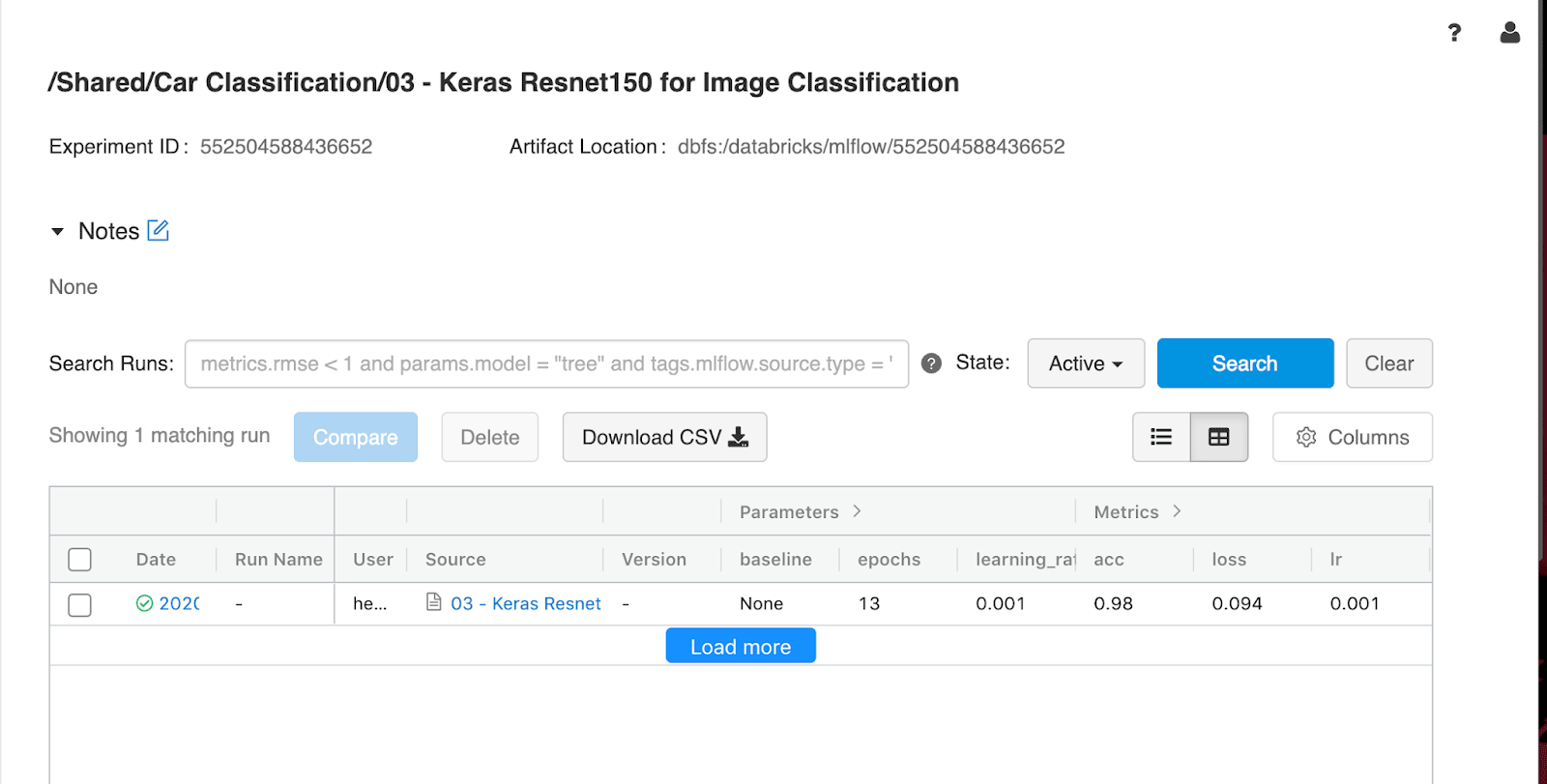
Machine learning development involves additional complexities beyond software development. That there are a myriad of tools and frameworks makes it hard to track experiments, reproduce results and deploy machine learning models. Together with Azure Machine Learning one can accelerate and manage the end-to-end machine learning lifecycle using MLflow to reliably build, share and deploy machine learning applications using Azure Databricks.
In order to automatically track results, an existing or new Azure ML workspace can be linked to your Azure Databricks workspace. Additionally, MLflow supports auto-logging for Keras models (mlflow.keras.autolog()), making the experience almost effortless.
While MLflow’s built-in model persistence utilities are convenient for packaging models from various popular ML libraries such as Keras, they do not cover every use case. For example, you may want to use a model from an ML library that is not explicitly supported by MLflow’s built-in flavours. Alternatively, you may want to package custom inference code and data to create an MLflow Model. Fortunately, MLflow provides two solutions that can be used to accomplish these tasks: Custom Python Models and Custom Flavors.
In this scenario we want to make sure we can use a model inference engine that supports serving requests from a REST API client. For this we are using a custom model based on the previously built Keras model to accept a JSON Dataframe object that has a Base64-encoded image inside.
In the next step we can use this py_model and deploy it to an Azure Container Instances server which can be achieved through MLflow’s Azure ML integration.
Deploy an Image Classification Model in Azure Container Instances
By now we have a trained machine learning model, and have registered a model in our workspace with MLflow in the cloud. As a final step we would like to deploy the model as a web service on Azure Container Instances.
A web service is an image, in this case a Docker image. It encapsulates the scoring logic and the model itself. In this case we are using our custom MLflow model representation which gives us control over how the scoring logic takes in care images from a REST client and how the response is shaped.
Container Instances is a great solution for testing and understanding the workflow. For scalable production deployments, consider using Azure Kubernetes Service. For more information, see how to deploy and where.
Getting Started with CNN Image Classification
This article and notebooks demonstrate the main techniques used in setting up an end-to-end workflow training and deploying a Neural Network in production on Azure. The exercises of the linked notebook will walk you through the required steps of creating this inside your own Azure Databricks environment using tools like Keras, Databricks Koalas, MLflow, and Azure ML.
Developer Resources
Get the latest posts in your inbox
Subscribe to our blog and get the latest posts delivered to your inbox.