Ensuring Quality Forecasts with Databricks Lakehouse Monitoring

Forecasting models are critical for many businesses to predict future trends, but their accuracy depends heavily on the quality of the input data. Poor quality data can lead to inaccurate forecasts that result in suboptimal decisions. This is where Databricks Lakehouse Monitoring comes in - it provides a unified solution to monitor both the quality of data flowing into forecasting models as well as the model performance itself.

Monitoring is especially crucial for forecasting models. Forecasting deals with time series data, where the temporal component and sequential nature of the data introduce additional complexities. Issues like data drift, where the statistical properties of the input data change over time, can significantly degrade forecast accuracy if not detected and addressed promptly.

Additionally, the performance of forecasting models is often measured by metrics like Mean Absolute Percentage Error (MAPE) that compare predictions to actual values. However, ground truth values are not immediately available, only arriving after the forecasted time period has passed. This delayed feedback loop makes proactive monitoring of input data quality and model outputs even more important to identify potential issues early.

Frequent retraining of statistical forecasting models using recent data is common, but monitoring remains valuable to detect drift early and avoid unnecessary computational costs. For complex models like PatchTST, which use deep learning and require GPUs, retraining may be less frequent due to resource constraints, making monitoring even more critical.

With automatic hyperparameter tuning, you can introduce skew and inconsistent model performance across runs. Monitoring helps you quickly identify when a model's performance has degraded and take corrective action, such as manually adjusting the hyperparameters or investigating the input data for anomalies. Furthermore, monitoring can help you strike the right balance between model performance and computational cost. Auto-tuning can be resource-intensive, especially if it's blindly running on every retraining cycle. By monitoring the model's performance over time, you can determine if the auto-tuning is actually yielding significant improvements or if it's just adding unnecessary overhead. This insight allows you to optimize your model training pipeline.

Databricks Lakehouse Monitoring is built to monitor the statistical properties and quality of data across all tables, but it also includes specific capabilities tailored for tracking the performance of machine learning models via monitoring inference tables containing model inputs and predictions. For forecasting models, this allows:

• Monitoring data drift in input features over time, comparing to a baseline
• Tracking prediction drift and distribution of forecasts
• Measuring model performance metrics like MAPE, bias, etc as actuals become available
• Setting alerts if data quality or model performance degrades

Creating Forecasting Models on Databricks

Before we discuss how to monitor forecasting models, let's briefly cover how to develop them on the Databricks platform. Databricks provides a unified environment to build, train, and deploy machine learning models at scale, including time series forecasting models.

There are several popular libraries and techniques you can use to generate forecasts, such as:

• Prophet: An open-source library for time series forecasting that is easy to use and tune. It excels at handling data with strong seasonal effects and works well with messy data by smoothing out outliers. Prophet's simple, intuitive API makes it accessible to non-experts. You can use PySpark to parallelize Prophet model training across a cluster to build thousands of models for each product-store combination. Blog
• ARIMA/SARIMA: Classic statistical methods for time series forecasting. ARIMA models aim to describe the autocorrelations in the data. SARIMA extends ARIMA to model seasonality. In a recent benchmarking study, SARIMA demonstrated strong performance on retail sales data compared to other algorithms. Blog

In addition to popular libraries like Prophet and ARIMA/SARIMA for generating forecasts, Databricks also offers AutoML for Forecasting. AutoML simplifies the process of creating forecasting models by automatically handling tasks like algorithm selection, hyperparameter tuning, and distributed training. With AutoML, you can:

• Quickly generate baseline forecasting models and notebooks through a user-friendly UI
• Leverage multiple algorithms like Prophet and Auto-ARIMA under the hood
• Automatically handle data preparation, model training and tuning, and distributed computation with Spark

You can easily integrate models created using AutoML with MLflow for experiment tracking and Databricks Model Serving for deployment and monitoring. The generated notebooks provide code that can be customized and incorporated into production workflows.

To streamline the model development workflow, you can leverage MLflow, an open-source platform for the machine learning lifecycle. MLflow supports Prophet, ARIMA and other models out-of-the-box to enable experiment tracking which is ideal for time series experiments, allowing for the logging of parameters, metrics, and artifacts. While this simplifies model deployment and promotes reproducibility, using MLflow is optional for Lakehouse Monitoring - you can deploy models without it and Lakehouse Monitoring will still be able to track them.

Once you have a trained forecasting model, you have flexibility in how you deploy it for inference depending on your use case. For real-time forecasting, you can use Databricks Model Serving to deploy the model as a low-latency REST endpoint with just a few lines of code. When a model is deployed for real-time inference, Databricks automatically logs the input features and predictions to a managed Delta table called an inference log table. This table serves as the foundation for monitoring the model in production using Lakehouse Monitoring.

However, forecasting models are often used in batch scoring scenarios, where predictions are generated on a schedule (e.g. generating forecasts every night for the next day). In this case, you can build a separate pipeline that scores the model on a batch of data and logs the results to a Delta table. It's more cost-effective to load the model directly on your Databricks cluster and score the batch of data there. This approach avoids the overhead of deploying the model behind an API and paying for compute resources in multiple places. The logged table of batch predictions can still be monitored using Lakehouse Monitoring in the same way as a real-time inference table.

If you do require both real-time and batch inference for your forecasting model, you can consider using Model Serving for the real-time use case and loading the model directly on a cluster for batch scoring. This hybrid approach optimizes costs while still providing the necessary functionality. You can leverage Lakeview dashboards to build interactive visualizations and share insights on your forecasting reports. You can also set up email subscriptions to automatically send out dashboard snapshots on a schedule.

Whichever approach you choose, by storing the model inputs and outputs in the standardized Delta table format, it becomes straightforward to monitor data drift, track prediction changes, and measure accuracy over time. This visibility is crucial for maintaining a reliable forecasting pipeline in production.

Now that we've covered how to build and deploy time series forecasting models on Databricks, let's dive into the key aspects of monitoring them with Lakehouse Monitoring.

Monitor Data Drift and Model Performance

To ensure your forecasting model continues to perform well in production, it's important to monitor both the input data and the model predictions for potential issues. Databricks Lakehouse Monitoring makes this easy by allowing you to create monitors on your input feature tables and inference log tables. Lakehouse Monitoring is built on top of Unity Catalog as a unified way to govern and monitor your data, and requires Unity Catalog to be enabled on your workspace.

Create an Inference Profile Monitor

To monitor a forecasting model, create an inference profile monitor on the table containing the model's input features, predictions, and optionally, ground truth labels. You can create the monitor using either the Databricks UI or the Python API.

In the UI, navigate to the inference table and click the "Quality" tab. Click "Get started" and select "Inference Profile" as the monitor type. Then configure the following key parameters:

• Problem Type: Select regression for forecasting models
• Timestamp Column: The column containing the timestamp of each prediction. It is the timestamp of the inference, not the timestamp of the data itself.
• Prediction Column: The column containing the model's forecasted values
• Label Column (optional): The column containing the actual values. This can be populated later as actuals arrive.
• Model ID Column: The column identifying the model version that made each prediction
• Granularities: The time windows to aggregate metrics over, e.g. daily or weekly

Optionally, you can also specify:

• A baseline table containing reference data, like the training set, to compare data drift against
• Slicing expressions to define data subsets to monitor, like different product categories
• Custom metrics to calculate, defined by a SQL expression
• Set up a refresh schedule

Using the Python REST API, you can create an equivalent monitor with code like:

from databricks.sdk import WorkspaceClient
from databricks.sdk.service.catalog import MonitorInferenceLog, 
MonitorInferenceLogProblemType, MonitorMetric, MonitorMetricType
from pyspark.sql import types as T

w = WorkspaceClient()

w.quality_monitors.create(
    table_name=f"{catalog}.{schema}.{table_name}",
    inference_log=MonitorInferenceLog(
        timestamp_col="ts",
        model_id_col="model_version",  
        prediction_col="prediction",
        label_col="actual",
        problem_type=MonitorInferenceLogProblemType.PROBLEM_TYPE_REGRESSION,
        granularities=["1 day", "1 week"]
    ),
    output_schema_name=f"{catalog}.{schema}",
    assets_dir= f"/Workspace/Users/{user_email}/databricks_lakehouse
    _monitoring/{catalog}.{schema}.{table_name}",
    baseline_table="my_training_table",
    slicing_exprs=["product_category"],
    custom_metrics=[
        MonitorMetric(
	     type=MonitorMetricType.CUSTOM_METRIC_TYPE_AGGREGATE,
            name="pct_within_tolerance",
     input_columns=[":table"], 
            definition="100.0 * sum(case when abs(prediction - actual) / 
            actual <= 0.1 then 1 else 0 end) / count(*)"
	     output_data_type=T.StructField("output", T.DoubleType()).json(),
        ),
        MonitorMetric(
	     type=MonitorMetricType.CUSTOM_METRIC_TYPE_AGGREGATE,
            name="weighted_mae", 
     input_columns=[":table"],
            definition="sum(abs(prediction - actual) * product_value) / 
            sum(product_value)"
	     output_data_type=T.StructField("output", T.DoubleType()).json(),
        ),
        MonitorMetric(
	     type=MonitorMetricType.CUSTOM_METRIC_TYPE_AGGREGATE,
            name="qoq_pct_change",
	     input_columns=[":table"],
            definition="""
                (sum(case when extract(quarter from ts) = extract(quarter 
                from current_timestamp) and extract(year from ts) = extract(
                year from current_timestamp) then actual else 0 end) /
                 nullif(sum(case when extract(quarter from ts) = extract(
                 quarter from current_timestamp) - 1 and extract(year from 
                 ts) = extract(year from current_timestamp) then actual else 
                 0 end), 0) - 1) * 100
            """
	     output_data_type=T.StructField("output", T.DoubleType()).json(),
        ),
    ]  
)

Baseline table is an optional table containing a reference dataset, like your model's training data, to compare the production data against. Again, for forecasting models, they are frequently retrained, so the baseline comparison is often not necessary as the model will frequently change. You may do the comparison to a previous time window and if baseline comparison is desired, only update the baseline when there is a bigger update, like hyperparameter tuning or an update to the actuals.

Monitoring in forecasting is useful even in scenarios where the retraining cadence is pre-set, such as weekly or monthly. In these cases, you can still engage in exception-based forecast management when forecast metrics deviate from actuals or when actuals fall out of line with forecasts. This allows you to determine if the underlying time series needs to be re-diagnosed (the formal forecasting language for retraining, where trends, seasonality, and cyclicity are individually identified if using econometric models) or if individual deviations can be isolated as anomalies or outliers. In the latter case, you wouldn't re-diagnose, but mark the deviation as an outlier and potentially attach a calendar event or an exogenous variable to the model in the future.

Lakehouse Monitoring will automatically track statistical properties of the input features over time and alert if significant drift is detected relative to the baseline or previous time windows. This allows you to identify data quality issues that could degrade forecast accuracy. For example:

• Monitor the distribution of key input features like sales amounts. If there is a sudden shift, it could indicate data quality issues that may degrade forecast accuracy.
• Track the number of missing or outlier values. An increase in missing data for recent time periods could skew forecasts.

In addition to the default metrics, you can define custom metrics using SQL expressions to capture business-specific logic or complex comparisons. Some examples relevant to forecasting:

• Comparing metrics across seasons or years, e.g. calculating the percent difference in average sales between the current quarter and the same quarter last year
• Weighting errors differently based on the item being forecasted, e.g. penalizing errors on high-value products more heavily
• Tracking the percentage of forecasts within an acceptable error tolerance

Custom metrics can be of three types:

• Aggregate metrics calculated from columns in the inference table
• Derived metrics calculated from other aggregate metrics
• Drift metrics comparing an aggregate or derived metric across time windows or to a baseline

Examples of these custom metrics are shown in the Python API example above. By incorporating custom metrics tailored to your specific forecasting use case, you can gain deeper, more relevant insights into your model's performance and data quality.

The key idea is to bring your model's input features, predictions, and ground truth labels together in one inference log table. Lakehouse Monitoring will then automatically track data drift, prediction drift, and performance metrics over time and by the dimensions you specify.

If your forecasting model is served outside of Databricks, you can ETL the request logs into a Delta table and then apply monitoring on it. This allows you to centralize monitoring even for external models.

It's important to note that when you first create a time series or inference profile monitor, it analyzes only data from the 30 days prior to the monitor's creation. Due to this cutoff, the first analysis window might be partial. For example, if the 30-day limit falls in the middle of a week or month, the full week or month will not be included.

This 30-day lookback limitation only affects the initial window when the monitor is created. After that, all new data flowing into the inference table will be fully processed according to the specified granularities.

Refresh Monitors to Update Metrics

After creating an inference profile monitor for your forecasting model, you need to periodically refresh it to update the metrics with the latest data. Refreshing a monitor recalculates the profile and drift metrics tables based on the current contents of the inference log table. You should refresh a monitor when:

• New predictions are logged from the model
• Actual values are added for previous predictions
• The inference table schema changes, such as adding a new feature column
• You modify the monitor settings, like adding additional custom metrics

There are two ways to refresh a monitor: on a schedule or manually.

To set up a refresh schedule, specify the schedule parameter when creating the monitor using the UI, or with the Python API:

from databricks.sdk import WorkspaceClient
from databricks.sdk.service.catalog import MonitorInferenceLog, 
MonitorInferenceLogProblemType, MonitorCronSchedule

w = WorkspaceClient()

w.quality_monitors.create(
    table_name=f"{catalog}.{schema}.{table_name}",
    inference_log=MonitorInferenceLog(...),
    schedule=MonitorCronSchedule(quartz_cron_expression="0 0 * * *")  
    # daily at midnight
    skip_builtin_dashboard=False  # set to True if dashboard is 
    already created
    output_schema_name=f"{catalog}.{schema}",
    assets_dir= f"/Workspace/Users/{user_email}/databricks_lakehouse
    _monitoring/{catalog}.{schema}.{table_name}",
)

The `CronSchedule` lets you provide a cron expression to define the refresh frequency, such as daily, hourly, etc. You can set `skip_builtin_dashboard` to True, which will skip generating a new dashboard for the monitor. This is especially useful when you have already built a dashboard or have custom charts in the dashboard you want to keep and don't need a new one.

Alternatively, you can manually refresh a monitor using the UI or Python API. In the Databricks UI, go to the "Quality" tab on the inference table, select the monitor, and click "Refresh metrics".

Using Python API, you can create a pipeline that refreshes a monitor so that it's action-driven, for example, after retraining a model. To refresh a monitor in a notebook, use the run_refresh function:

from databricks.sdk import WorkspaceClient

w = WorkspaceClient()

w.quality_monitors.run_refresh(
    table_name=f"{catalog}.{schema}.{table_name}"
)

This submits a serverless job to update the monitor metrics tables. You can continue to use the notebook while the refresh runs in the background.

After a refresh completes, you can query the updated profile and drift metrics tables using SQL. However, note that the generated dashboard is updated separately, which you can do so by clicking on the "Refresh" button in the DBSQL dashboard itself. Similarly, when you click Refresh on the dashboard, it doesn't trigger monitor calculations. Instead, it runs the queries over the metric tables that the dashboard uses to generate visualizations. To update the data in the tables used to create the visualizations that appear on the dashboard, you must refresh the monitor and then refresh the dashboard.

Understanding the Monitoring Output

When you create an inference profile monitor for your forecasting model, Lakehouse Monitoring generates several key assets to help you track data drift, model performance, and overall health of your pipeline.

Profile and Drift Metrics Tables

Lakehouse Monitoring creates two primary metrics tables:

1. Profile metrics table: Contains summary statistics for each feature column and the predictions, grouped by time window and slice. For forecasting models, this includes metrics like:
   • count, mean, stddev, min, max for numeric columns
   • count, number of nulls, number of distinct values for categorical columns
   • count, mean, stddev, min, max for the prediction column
2. Drift metrics table: Tracks changes in data and prediction distributions over time compared to a baseline. Key drift metrics for forecasting include:
   • Wasserstein distance for numeric columns, measuring the difference in distribution shape, and for the prediction column, detecting shifts in the forecast distribution
   • Jensen-Shannon divergence for categorical columns, quantifying the difference between probability distributions

You can query them directly using SQL to investigate specific questions, such as:

• What is the average prediction and how has it changed week-over-week?
• Is there a difference in model accuracy between product categories?
• How many missing values were there in a key input feature yesterday vs the training data?

Model Performance Dashboard

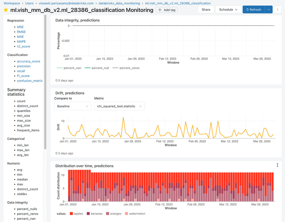
In addition to the metrics tables, Lakehouse Monitoring automatically generates an interactive dashboard to visualize your forecasting model's performance over time. The dashboard includes several key components:

1. Model Performance Panel: Displays key accuracy metrics for your forecasting model, such as MAPE, RMSE, bias, etc. These metrics are calculated by comparing the predictions to the actual values, which can be provided on a delay (e.g. daily actuals for a daily forecast). The panel shows the metrics over time and by important slices like product category or region.
2. Drift Metrics Panel: Visualizes the drift metrics for selected features and the prediction column over time.
3. Data Quality Panel: Shows various metrics such as % of missing values, % of nas, various statistics such as count, mean, min and max, and other data anomalies for both numeric features and categorical features over time. This helps you quickly spot data quality issues that could degrade forecast accuracy.

The dashboard is highly interactive, allowing you to filter by time range, select specific features and slices, and drill down into individual metrics. The dashboard is often customized after its creation to include any views or charts your organization is used to looking at. Queries that are used on the dashboard can be customized and saved, and you can add alerts from any of the views by clicking on "view query" and then clicking on "create alert". At the time of writing, a customized template for the dashboard is not supported.

It's a valuable tool for both data scientists to debug model performance and business stakeholders to maintain trust in the forecasts.

Leveraging Actuals for Accuracy Monitoring

To calculate model performance metrics like MAPE, the monitoring system needs access to the actual values for each prediction. However, with forecasting, actuals are often not available until some time after the prediction is made.

One strategy is to set up a separate pipeline that appends the actual values to the inference log table when they become available, then refresh the monitor to update the metrics. For example, if you generate daily forecasts, you could have a job that runs each night to add the actual values for the previous day's predictions.

By capturing actuals and refreshing the monitor regularly, you can track forecast accuracy over time and identify performance degradation early. This is crucial for maintaining trust in your forecasting pipeline and making informed business decisions.

Moreover, monitoring actuals and forecasts separately enables powerful exception management capabilities. Exception management is a popular technique in demand planning where significant deviations from expected outcomes are proactively identified and resolved. By setting up alerts on metrics like forecast accuracy or bias, you can quickly spot when a model's performance has degraded and take corrective action, such as adjusting model parameters or investigating input data anomalies.

Lakehouse Monitoring makes exception management straightforward by automatically tracking key metrics and providing customizable alerting. Planners can focus their attention on the most impactful exceptions rather than sifting through mountains of data. This targeted approach improves efficiency and helps maintain high forecast quality with minimal manual intervention.

In summary, Lakehouse Monitoring provides a comprehensive set of tools for monitoring your forecasting models in production. By leveraging the generated metrics tables and dashboard, you can proactively detect data quality issues, track model performance, diagnose drift, and manage exceptions before they impact your business. The ability to slice and dice the metrics across dimensions like product, region, and time enables you to quickly pinpoint the root cause of any issues and take targeted action to maintain the health and accuracy of your forecasts.

Set Alerts on Model Metrics

Once you have an inference profile monitor set up for your forecasting model, you can define alerts on key metrics to proactively identify issues before they impact business decisions. Databricks Lakehouse Monitoring integrates with Databricks SQL to allow you to create alerts based on the generated profile and drift metrics tables.

Some common scenarios where you would want to set up alerts for a forecasting model include:

• Alert if the rolling 7-day average prediction error (MAPE) exceeds 10%. This could indicate the model is no longer accurate and may need retraining.
• Alert if the number of missing values in a key input feature has increased significantly compared to the training data. Missing data could skew predictions.
• Alert if the distribution of a feature has drifted beyond a threshold relative to the baseline. This could signal a data quality issue or that the model needs to be updated for the new data patterns.
• Alert if no new predictions have been logged in the past 24 hours. This could mean the inference pipeline has failed and needs attention.
• Alert if the model bias (mean error) is consistently positive or negative. This could indicate the model is systematically over or under forecasting.

There are built-in queries already generated to build the views of the dashboard. To create an alert, navigate to the SQL query that calculates the metric you want to monitor from the profile or drift metrics table. Then, in the Databricks SQL query editor, click "Create Alert" and configure the alert conditions, such as triggering when the MAPE exceeds 0.1. You can set the alert to run on a schedule, like hourly or daily, and specify how to receive notifications (e.g. email, Slack, PagerDuty).

In addition to alerts on the default metrics, you can write custom SQL queries to calculate bespoke metrics for your specific use case. For example, maybe you want to alert if the MAPE for high-value products exceeds a different threshold than for low-value products. You could join the profile metrics with a product table to segment the MAPE calculation.

The key is that all the feature and prediction data is available in metric tables, so you can flexibly compose SQL to define custom metrics that are meaningful for your business. You can then create alerts on top of these custom metrics using the same process.

By setting up targeted alerts on your forecasting model metrics, you can keep a pulse on its performance without manual monitoring. Alerts allow you to respond quickly to anomalies and maintain trust in the model's predictions. Combined with the multi-dimensional analysis enabled by Lakehouse Monitoring, you can efficiently diagnose and resolve issues to keep your forecast quality high.

Monitor Lakehouse Monitoring Expenses

While not specific to forecasting models, it's important to understand how to track your usage and expenses for Lakehouse Monitoring itself. When planning to use Lakehouse Monitoring, it's important to understand the associated costs so you can budget appropriately. Lakehouse Monitoring jobs run on serverless compute infrastructure, so you don't have to manage clusters yourself. To estimate your Lakehouse Monitoring costs, follow these steps:

1. Determine the number and frequency of monitors you plan to create. Each monitor will run on a schedule to refresh the metrics.
2. Estimate the data volume and complexity of the SQL expressions for your monitors. Larger data sizes and more complex queries will consume more DBUs.
3. Look up the DBU rate for serverless workloads based on your Databricks tier and cloud provider.
4. Multiply your estimated DBUs by the applicable rate to get your estimated Lakehouse Monitoring cost.

Your actual costs will depend on your specific monitor definitions and data, which can vary over time. Databricks provides two ways to monitor your Lakehouse Monitoring costs: using a SQL query or the billing portal. Refer to https://docs.databricks.com/en/lakehouse-monitoring/expense.html for more information.

Ready to start monitoring your forecasting models with Databricks Lakehouse Monitoring? Sign up for a free trial to get started. Already a Databricks customer? Check out our documentation to set up your first inference profile monitor today.